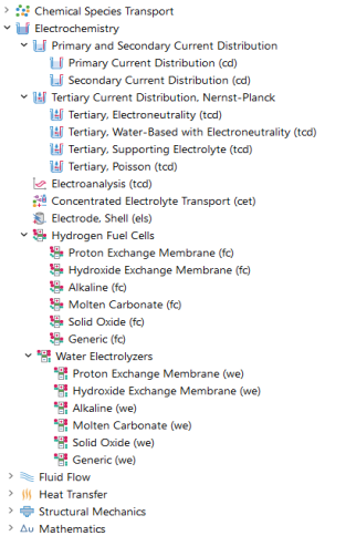
Figure 3 below shows the Fuel Cell & Electrolyzer Module interfaces, in the Electrochemistry branch, as displayed in the Model Wizard for a 3D model.

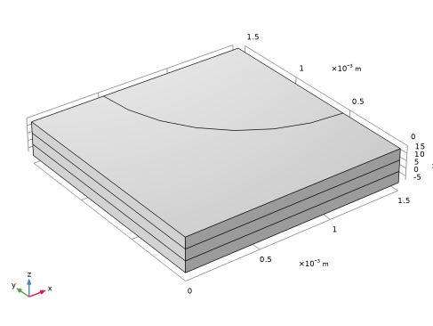
Figure 4 shows an example 3D geometry of a cathode from a fuel cell with perforated current collectors. This geometry configuration can be used for self-breathing cathodes or in small experimental cells. Due to the perforation layout, a 3D model is needed in the study of the mass transport, current, and reaction distributions.

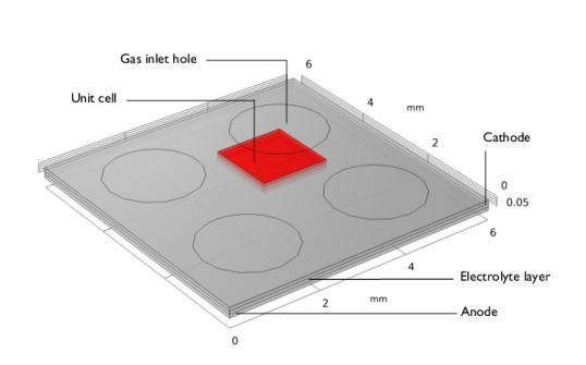
Figure 5 shows details for a unit cell, cut out from Figure 4. (In this case, the combination of a circular orifice and square unit cell eliminates the possibility to approximate the geometry with a rotationally symmetric model.) The circular hole in the collector acts as an inlet where the gas enters the modeling domain, and at this boundary the gas mixture composition and pressure is known. The upper and lower rectangular domains are the reaction-zone gas diffusion electrodes. They consist of a three-phase porous structure that contains the feed-gas mixture, an electronically conducting material covered with an electrocatalyst, and an ionically conducting electrolyte.

The Hydrogen Fuel Cell interface models the electronic and ionic current balances and solves for the potentials ϕs and ϕl in the electrode and electrolyte phases, respectively. The anode side of the cell is grounded, whereas the current collector boundary at the cathode is set to a cell potential value.

The species (mass) transport is modeled by the Maxwell–Stefan equations for the mass fractions of oxygen, water, and nitrogen in the O2 gas phase. Mass transport is solved for in the cathode gas diffusion electrode domain only. Similarly, the pressure and the resulting velocity vector is solved for in the cathode gas diffusion electrode domain only using Darcy’s Law. (No mass transport effects are expected to occur at the hydrogen anode side). As boundary conditions, inlet molar fractions are set for the three gas species corresponding to a humidified air mixture at 90% relative humidity at atmospheric pressure.

where T denotes the temperature, n the number of electrons participating in the electrode reaction, and F Faraday’s constant.

where νi are the stoichiometric coefficients of the reacting species.

where pi is the partial pressure of the reacting species, pref = 1 atm is the reference pressure and ηref, the overpotential with respect to the reference state, is defined as

The local current density expression in the cathode is multiplied by a specific area of 109 m2/m3 to create a volumetric current source term in the electrode domain. Assuming ideal kinetics according to the mass action law, αa,O2 + αc,O2 = n.

assuming αa,H2 + αc,H2 = n and where, since the anode boundary is grounded, the overpotential is defined as

In the first part of the model instruction below, a secondary (not concentration dependent) current distribution is modeled. In the second part, mass, and momentum transport is incorporated in the O2 gas phase mixture (cathode domain), using Maxwell–Stefan diffusion and Darcy’s Law, respectively. In both parts of the tutorial, the model is solved for a range of cell potential values (0.5 V to 1 V in steps of 0.1 V) by the use of an auxiliary sweep in the stationary solver.

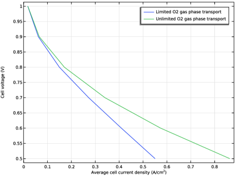
Figure 6 shows the polarization plot for the two scenarios investigated: limited and unlimited O2 gas phase transport. It can be seen that higher average cell current densities are achieved for the unlimited O2 gas phase transport scenario (that is, when no mass and momentum transport limitations are present).

Note that the plots and discussion in the rest of this section correspond to the limited O2 gas phase transport scenario, where diffusion and flow (in the cathode domain) have been considered, coupled to charge transport and the electrochemical reactions.

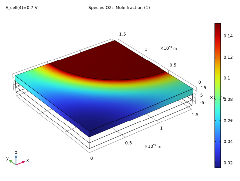
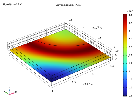
Figure 7 shows the oxygen mole fraction at cell voltage of 0.7 V. The figure shows that mole fraction variations are small along the thickness of the cathode, while they are substantially larger along the electrode’s width.

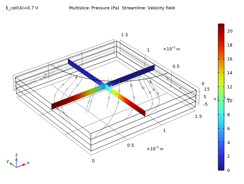
Figure 8 shows the pressure and gas velocity streamlines in the porous cathode at the same cell voltage. There is a significant velocity peak at the edge of the inlet orifice. This is caused by the contributions of the reactive layer underneath the current collector because in this region the convective flux dominates the mass transport. The gas flows from the interior of the cell toward the circular hole. The reason for this is the oxygen reduction reaction, with the creation of two water gas molecules, being transported out of the cell, per oxygen molecule entering the cell.

The electrochemical reaction rate, represented by the local current density, is related to both the local overpotential and oxygen concentration in the cathode domain. Figure 9 depicts the local overpotential (at cell voltage of 0.7 V), which gets more negative toward the electrolyte domain.

The combination of the overpotential and oxygen concentration distributions will result in a highly uneven reaction rate in the reactive layer. One way to study the distribution of the reaction rate is to plot the ionic current density at the bottom boundary of the membrane layer. Figure 10 shows such a plot at cell voltage of 0.7 V.

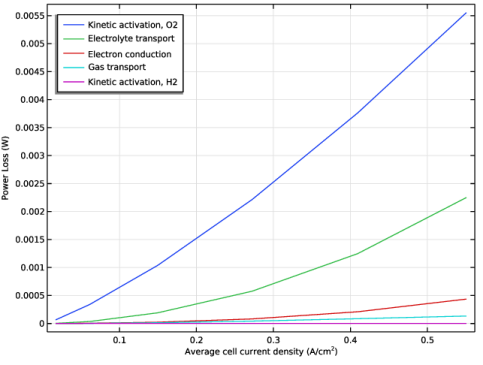
Figure 11 shows a plot of the cell-integrated power losses associated with the different processes in the cell. For this cell, the power losses due to kinetic activation of the oxygen reduction reaction dominate the losses, followed by the electrolyte transport losses.

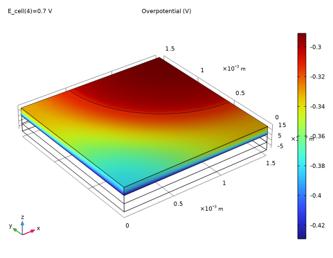
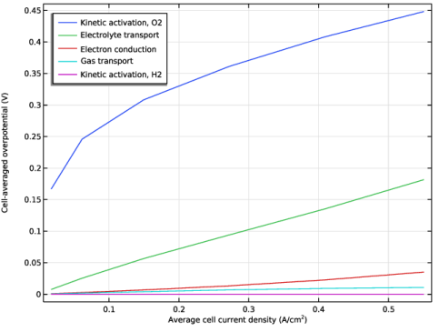
By dividing the loss in power by the cell current, we can also compute the corresponding cell overpotentials, as shown in Figure 12. The oxygen reduction overpotential is highly nonlinear with respect to the cell current density. This stems from the Butler-Volmer kinetics deployed in the model. The electrolyte transport overpotential has a more linear behavior with respect to the cell current density.