Tutorial — Copper Deposition in a Trench
This model simulates the electroplating of copper in a microcavity typically found in the plating of copper onto circuit boards. The plating cell is a laboratory cell under potentiostatic control where the anode is placed in close vicinity of the cathode. The model is based on the work by Mattsson and Bockris (Ref. 1).
The purpose of the model is to demonstrate the use of moving meshes for plating processes and to investigate the influence of the cavity on the plating result. The moving mesh makes it possible to simulate the growth of the cathode boundary as the process proceeds.
Model Definition
The model simulates the deposition process at pH 4, which implies that the proton concentration is very low compared to the copper and sulfate ion concentrations. For this reason, the material balance of the protons does not need to be modeled. Sulfate is also treated as a fully dissociated ion. The deposition at the cathode and the dissolution at the anode are assumed to take place with 100% current yield, which means that the model does not include possible side reactions. During the process, differences in electrolyte density arise in the enclosed cell, giving higher density at the anode compared to the cathode. This can induce free convection in the cell. Under the modeled conditions, however, the variations in composition are small and it is therefore possible to neglect free convection.
The process is inherently time-dependent because the cathode boundary moves as the deposition process takes place. The model is defined by the material balances for the involved ions — copper, Cu2+, and sulfate, SO42- — and the electroneutrality condition. This gives three unknowns and three model equations. The dependent variables are the copper ion, sulfate ion, and ionic potentials. Additional variables keep track of the deformation of the mesh.
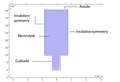
The model geometry is shown in Figure 5. The upper horizontal boundary represents the anode, while the cathode is placed at the bottom. The vertical walls correspond to the pattern on the master electrode and are assumed to be insulating.
Figure 5: Model domain with boundaries corresponding to the anode, cathode, and vertical symmetry walls.
The flux for each of the ions in the electrolyte is given by the Nernst–Planck equation
(11)
where Ji denotes the transport vector (mol/(m2·s)), ci the concentration in the electrolyte (mol/m3), zi the charge for the ionic species, ui the mobility of the charged species (m2/(s·J·mole)), F Faraday’s constant (A·s/mole), and the potential in the electrolyte (V). The material balances are expressed through
(12)
one for each species, that is i = 1, 2. The electroneutrality condition is given by the following expression:
(13)
The boundary conditions for the anode and cathode are given by the Butler–Volmer equation for copper deposition. The deposition process is assumed to take place through the following simplified mechanism:
(14)
where the first step is rate determining step, RDS, and the second step is assumed to be at equilibrium (Ref. 1). This gives the following relation for the local current density as a function of potential and copper concentration:
(15)
where η denotes the overpotential defined as
(16)
where denotes the electronic potential of the respective electrode. This gives the following condition for the cathode:
(17)
where n denotes the normal vector to the boundary. The condition at the anode is
(18)
All other boundaries are insulating:
(19)
For the sulfate ions, insulating conditions apply everywhere:
(20)
The initial conditions set the composition of the electrolyte according to
(21)
You set up Equation 11 through Equation 21 using the Tertiary Current Distribution, Nernst–Planck interface. The Deformed Geometry interface keeps track of the deformation of the mesh.
Using the Electrode Surface boundary node, the ion fluxes and the boundary mesh velocity are based on the reaction currents, the number of electrons, and the specified stoichiometric coefficients of the electrode reactions. The sign of the stoichiometric coefficient for a species depends on whether the species is getting oxidized (positive) or reduced (negative) in the reaction. In the case for the total reaction in this model
the stoichiometric coefficient is for the copper ions in the electrolyte, and for the copper atoms in the electrodes.
Results and Discussion
Figure 6 shows the concentration distribution of copper ions, the isopotential lines, the current density lines, and the displacement of the cathode and anode surfaces after 14 seconds of operation. The figure shows that the mouth of the cavity is narrower due to the nonuniform thickness of the deposition. This effect can be detrimental to the quality of the deposition because a trapped electrolyte can later cause corrosion of components in the circuit board. In addition, the simulation shows substantial variations in copper ion concentration in the cell. Such variations eventually cause free convection in the cell. The model is symmetric along a vertical line in the middle of the cell. A nonsymmetric result is a sign of poor mesh resolution.
Figure 6: Copper ion concentration (mol/m3), isopotential lines, current density streamlines, and electrode displacement in the cell after 14 seconds of operation.
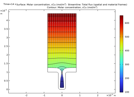
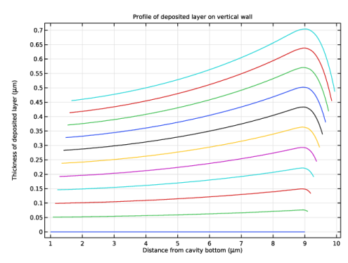
Figure 7 shows the thickness of the deposition along one of the vertical cathodic surfaces. The lines reveal the development of the nonuniform deposition due to nonuniform current density distribution. This effect is accentuated by the depletion of copper ions along the depth of the cavity.
Figure 7: Thickness of the deposition along the vertical cathode boundaries. The lines are generated for increments of 0.5 seconds from 0 to 5 seconds.
Despite the simplicity of this model, it can easily be expanded to more complicated geometries or to include the influence of more ions on the process.
Reference
1. E. Mattsson and J.O’M. Bockris, “Galvanostatic Studies of the Kinetics of Deposition and Dissolution in the Copper + Copper Sulphate System,” Trans. Far. Soc., vol. 55, p. 1586, 1959.