Tutorial — Decorative Plating
This electroplating model uses secondary current distribution with full Butler–Volmer kinetics for the metal deposition or dissolution reaction on the cathode and anode. A competing hydrogen evolution reaction is also present on the cathode. The thickness of the deposited layer at the cathode is computed as well as the current efficiency.
Model Definition
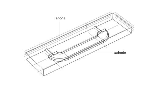
The model geometry is shown in Figure 4. The anode is a planar dissolving anode. The cathode represents a furniture fitting that is to be decorated by metal plating.
Figure 4: The model geometry.
The conductivity of the metal of the anode and cathode is very high compared to that of the electrolyte, and it is assumed that the electric potential in the metal is constant. The variations in the activation overpotential are therefore caused by the potential in the electrolyte at the surface of the electrodes. Under these assumptions, the electrodes are treated as boundaries in the simulations.
Before beginning, one difficulty found in all current density distribution models needs to be discussed.
The overpotential, η m, for an electrode reaction of index m, is defined according to the following equation:
(1)
where ϕs,0 denotes the electric potential of the metal, ϕl denotes the potential in the electrolyte, and 
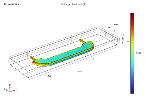
Eeq,m denotes the difference between the metal and electrolyte potentials at the electrode surface measured at equilibrium using a common reference potential. The electric potential of one of the electrodes may be bootstrapped, so that all other potentials are measured with this reference (this bootstrap can actually be achieved by fixing the potential at any point in the cell). In this case, the electric potential of the metal is selected at the cathode as a bootstrap by setting this potential to 0 V. This implies that the electric potential of the metal at the anode is equal to the cell voltage. The potential of the electrolyte floats and adapts to satisfy the balance of current, so that an equal amount of current that leaves at the cathode also enters at the anode. This then determines the overpotential at the anode and the cathode.
Electrolyte charge transport
Use the Secondary Current Distribution interface to solve for the electrolyte potential, ϕl(V), assuming bulk electroneutrality:
(2)
where il (A/m2) is the electrolyte current density vector and σl (S/m) is the electrolyte conductivity, which is assumed to be a constant.
Use the default Insulation condition for all boundaries except the anode and cathode surfaces:
(3)
where n is the normal vector, pointing out of the domain.
The main electrode reaction on both the anode and the cathode surfaces is the nickel deposition/dissolution reaction according to
(4)
Using the Butler–Volmer equation to model this reaction will set the local current density to
(5)
The rate of deposition at the cathode boundary surfaces and the rate of dissolution at the anode boundary surface, with a velocity in the normal direction, v (m/s), is calculated according to
(6)
where M is the mean molar mass (59 g/mol) and ρ is the density (8900 kg/m3) of the nickel atoms and 
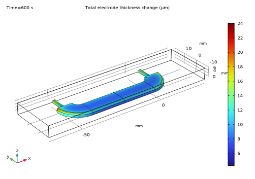
n is number of participating electrons. It should be noted that the local current density is positive at the anode surface and it is negative at the cathode surfaces.
On the anode the electrolyte current density is set to the local current density of the nickel deposition reaction:
(7)
On the cathode, add a second electrode reaction to model the parasitic hydrogen evolution reaction:
(8)
Using cathodic Tafel equation to model the kinetics of the hydrogen reaction on the cathode will set the local current density to
(9)
The hydrogen reaction will not contribute to the rate of deposition of nickel, but it will contribute to the total current density at the cathode surface:
(10)
Solve the model in a time-dependent study, simulating the electroplating for 600 s.
Results
The figure below shows the thickness of the deposited layer after 600 s of deposition. The variations in thickness are relatively large, more than a factor of 5 between the thinnest and thickest parts. This suggests the need for an improvement of the cell geometry. Another alternative is to add surface active species, also called levelers, that increase the kinetic losses at the electrode surfaces. These levelers help maintain a uniform current density.
The second figure, shown below, depicts the local current efficiency over the cathode surface. The efficiency is calculated as the nickel deposition current density divided by the total current density at the cathode and is around 97%.