COMSOL 6.4 - Results

The model is now solved and default plots are added. Follow the remaining steps below to reproduce the plots from the Results and Discussion section.

1D Plot Group 6 (Rebar Electrode-Electrolyte Potential)

1

In the Home toolbar click Add Plot Group

and choose 1D Plot Group

2

On the 1D Plot Group 6 toolbar click Point Graph

3

In the Model Builder click Point Graph 1

4

Select Points 3, 4, and 5 only. These points are on the edge of the rebar.

5

In the Settings window for Point Graph, click Replace Expression

in the upper-right corner of the y-axis data section. From the menu, choose Model > Component 1 > Tertiary Current Distribution, Nernst–Planck > tcd.Evsref - Electrode potential vs adjacent reference.

6

Click to expand the Legends section. Select the Show legends checkbox.

7

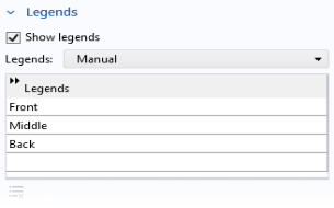
From the Legends list choose Manual. In each row of the table, enter Front, Middle, and Back as in the figure.

8

In the Model Builder click the 1D Plot Group 6

node. Press F2 and rename the node Rebar potential.

9

Click the Plot button

. Your plot should look like the one in Figure 9.

Next, add four more 1D Plot Groups. Except for the Expression selected or entered, the plots are similar. Duplicating the already created nodes reduces the number of required steps.

1D Plot Group 7(Oxygen Concentration)

1

Right-click Rebar potential

(the third plot group node) and choose Duplicate

2

Click Rebar potential 1

3

Go to the Rename 1D Plot Group dialog and type Oxygen concentration in the New name text field. Click OK.

4

In the Model Builder expand the Results > Oxygen concentration node then click Point Graph 1

5

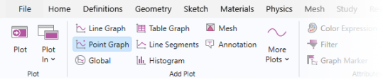
In the Settings window for Point Graph click Replace Expression

(it is in the upper-right corner of the y-axis data section). Choose .

6

Click the Plot button

. Your plot should look like the one in Figure 10.

1D Plot Group 8 (Oxygen Reduction Current Density)

1

In the Model Builder right-click Oxygen concentration

and choose Duplicate

2

Click Oxygen concentration 1

3

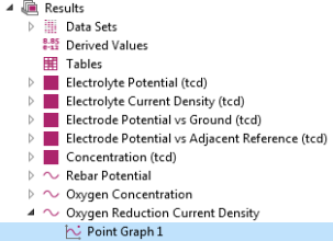
Go to the Rename 1D Plot Group dialog and type Oxygen Reduction Current Density in the New name text field and click OK.

4

In the Model Builder expand the Results > Oxygen reduction currents node then click Point Graph 1

5

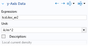
In the Settings window of the y-axis data section click Replace Expression

6

Click the Plot button

to update the plot in the Graphics window. Your plot should look like the one in Figure 11.

1D Plot Group 9 (Iron Oxidation Current Density)

1

In the Model Builder right-click Oxygen Reduction Current Density

and choose Duplicate

2

Click Oxygen Reduction Current Density 1

3

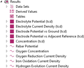
Go to the Rename 1D Plot Group dialog and type Iron Oxidation Current Density in the New name text field. Click OK.

4

In the Model Builder expand the Results > Iron Oxidation Current Density node, then click Point Graph 1

5

In the Settings window of the y-axis section click Replace Expression

6

Click the Plot button

to update the plot in the Graphics window. Your plot should look like the one in Figure 13.

1D Plot Group 10 (Hydrogen Evolution Current Density)

1

In the Model Builder right-click Iron Oxidation Current Density

and choose Duplicate

2

Click Iron Oxidation Current Density 1

3

Go to the Rename 1D Plot Group dialog and type Hydrogen Evolution Current Density in the New name text field. Click OK.

4

In the Model Builder expand the Results > Hydrogen Evolution Current Density node, then click Point Graph 1

5

In the Settings window of the y-axis section click Replace Expression

and choose from the menu.

6

Click the Plot button

to update the plot in the Graphics window. Your plot should look like the one in Figure 12.

The final set of plots under Results should match the following figure.