Running a study, on the other hand, can be different. When you compute a Study, it runs the solver configuration or creates a new one (see below). What the Study runs can be a Job or a Solver sequence (for example, a Stationary Solver) depending on the study configuration. If a Job (Subnode) is run, it typically also means that a solver is also run (by the job). But before the study runs a job or a solver, it reconstructs the configurations from scratch. An exception to this rule is when the configurations are edited (an asterisk indicates this; see Figure 20-7 for an example), in which case the sequences are computed “as is.”

Only one sequence per study can be run when computing the study. You can choose to exclude a sequence when computing a study by right-clicking the node and selecting Exclude When Computing Study (). An icon () indicates which sequences are excluded. If you want to run an excluded sequence when computing the study, right-click the node and select Run When Computing Study () — this excludes all other sequences in the particular study. If all sequences are excluded when the study is computed, a new sequence with default settings is generated.

If there is a top-level node under Job Configurations that is set to run when computing the study, it assumes control over the running of solver sequences to which it refers. For example, the solver sequence selected in a Solution node under a Parametric Sweep job cannot be excluded when computing the study. Conversely, if one in this situation chooses Run When Computing Study for some other solver sequence, then that sequence will also be automatically selected in the Solution nodes under any Parametric Sweep job set to run when computing the study.

Also see Figure 20-6 for other examples of excluded sequences.

The most straightforward method to compute a solution is to right-click the Study node () and select Compute () or press F8. You can also click Compute () in the main and Study toolbars and in the toolbar at the top of the study steps’ and solver nodes’ Settings windows.

By default, a study creates a Solution dataset and plot groups with results plots suitable for the physics interfaces for which you compute the solution. If you do not want to generate plots automatically, clear the Generate default plots checkbox in the Study Settings section in the main Study node’s Settings window. You can also right-click the main Study node and select Show Default Plots () from the Plots submenu to add the plot groups and plots that are added by default if the Generate default plots checkbox is selected. Right-click the main Study node and choose Reset Default Plots () from the Plots submenu to restore the default plots and their settings to the default plots and settings if you have changed or removed the default plots.

If you show the solver sequences under Solver Configurations, you can right-click any node in a solver sequence and select:

To update the solution for a study to use the current values of parameters and user-defined variables, right-click the Study node and select Update Solution () (or press F5). This is useful in the following situations when you have:

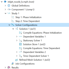
When you have added study steps to a study, a solver configuration or solver sequence is generated and added to Solver Configurations when the Study is computed. If the study contains auxiliary steps, for example Parametric Sweep, a job sequence may also be generated under Job Configurations. The solver sequence represents the steps required for computing a solution corresponding to each study step, including compiling all equations, initializing the solution and solving the discretized model.

In some cases, the default solver settings generated based on the study step settings are not sufficient to specify the details of how to obtain a solution. In this case you can edit the solver sequence and run it again. See Editing and Rerunning a Solver Configuration below.

For example, right-click a Dependent Variables node and select Run to Selected to evaluate the initial values for the dependent variables (similar to the Get Initial Value and Get Initial Value for Step options for the main Study nodes and the study steps).

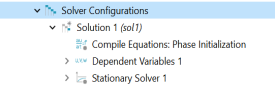
The Solver Configurations branch nodes (or if applicable, the Job Configurations branch) can be edited to adjust solver settings, for example, if you want to change a tolerance or use a different time-stepping method. If you edit any settings in a subnode to a Solution node, an asterisk in the upper-right corner (Figure 20-8) indicates that the settings differ from the default settings based on the study steps in the study.

To see what properties and values that have changed in any node with an asterisk in a solver configuration, the Changes from Default Values section at the bottom of each node’s Settings window contains a list of all properties that have changed, including descriptions, property names, default values, and current values.

After editing a solver configuration, you run the sequence again. Running a solver configuration is tantamount to computing a solution. Like mesh nodes, solution nodes are not built automatically as they are added. It is possible to have several solver configurations under a Solver Configurations node (see Figure 20-7), including Solution - Copy nodes for copies of a solution (see Create Solution Copy).

Under Cluster Computing, you get information about cluster solution storage. You can also choose a partitioning method from the Partitioning method for distributed computing list: Off (the default), Mesh ordering, Nested dissection, or Weighted nested dissection. This method affects the partitioning of the mesh data on cluster for the purpose of creating a DOF enumeration optimized for the particular cluster configuration (number of nodes). Mesh ordering is doing the partitioning based on existing mesh-element order and will produce a result similar to the existing DOF enumeration without any partitioning of the data. The nested dissection will on n cluster nodes partition the mesh data into n parts, minimizing the overlap between the parts before the DOFs for all the parts are enumerated. The weighted nested dissection option takes into account the expected number of DOFs per mesh element to produce parts with comparable total number of DOFs in each part. The benefit of using nested dissection and weighted nested dissection partitioning for cluster configuration-specific DOF enumeration is the performance improvement due to the reduction in the amount of communication between cluster nodes.

Right-click a Solution node and choose Domain Decomposition > Convert to Domain Decomposition (Schwarz) and Domain Decomposition > Convert to Domain Decomposition (Schur) to convert a solver into a similar Domain Decomposition solver with settings adapted for cluster computing. These options for conversion to domain decomposition solvers are also available on the context menus of solver nodes that support direct and iterative solvers (such as Stationary Solver and Time-Dependent Solver nodes). They are mainly intended for running on larger clusters where the domain decomposition strategy can be faster than the usual solvers. See Domain Decomposition (Schwarz) and Domain Decomposition (Schur) for more information about the domain decomposition solvers.

While a problem is being solved, it is useful to know its progress. The Progress Window monitors the state of the analysis for the solvers during the solution process. In this window, you can Cancel or Stop a Solver Process and also continue the solver process. Alternatively, in The Log Window you can inspect convergence information and other data from the latest and earlier runs.