COMSOL 6.4 - Accessing System Matrices and Vectors

Accessing System Matrices and Vectors

You can gain low-level access to the finite element system matrices and vectors by adding nodes of the types Assemble and Input Matrix under a Study node.

The example below shows how to set up and solve a 2D electrostatics problem on the unit square [0,1]-by-[0,1]. After the original problem is solved, the load vector is modified at a user-defined coordinate. The code searches for the degree of freedom closest to the target user-defined coordinate and modifies the load vector to a user-defined value. The physical interpretation of the modified load is that of an added volume charge.

To run the example code below, first use the Model Wizard to create a blank model. Then, add a new method and paste the example code below. Finally, run the method. You can try changing the variable values in the Initializations section at the beginning of the code and run again.

// Initializations

double x_load = 0.2; // Target x-coordinate for load

double y_load = 0.2; // Target y-coordinate for load

double load = 1e-9; // Load, volume charge

double dist = 10.0; // Distance to (x_load,y_load) from degree of freedom

int index = 0; // Index of the degree of freedom closest to (x_load,y_load)

// Clear any previous model

clearModel(model);

// Create a new model component

model.modelNode().create("comp1");

// Create the 2D geometry

model.geom().create("geom1", 2);

model.geom("geom1").feature().create("sq1", "Square");

model.geom("geom1").run();

// Create the mesh

model.mesh().create("mesh1", "geom1");

model.mesh("mesh1").feature().create("fre1", "FreeTri");

model.mesh("mesh1").run();

// Setup the electrostatics physics problem

model.physics().create("es", "Electrostatics", "geom1");

model.physics("es").feature().create("gnd1", "Ground", 1);

model.physics("es").feature("gnd1").selection().set(new int[]{1});

model.physics("es").feature().create("sfcd1", "SurfaceChargeDensity", 1);

model.physics("es").feature("sfcd1").selection().set(new int[]{4});

// Add a varying distributed charge density along the rightmost boundary

model.physics("es").feature("sfcd1").set("rhoqs", "1e-9*y");

// The following two lines using the ccn1 feature are only needed in version 6.2 and earlier versions

//model.component("comp1").physics("es").feature("ccn1").set("epsilonr_mat", "userdef");

//model.component("comp1").physics("es").feature("ccn1").set("epsilonr", "1");

// Change to first-order shape functions, to keep things simple

model.component("comp1").physics("es").prop("ShapeProperty").

set("order_electricpotential", 1);

// Create and run the study.

model.study().create("std1");

model.study("std1").feature().create("stat1", "Stationary");

model.study("std1").run();

// Create a 2D plot group with a surface plot for the original problem

model.result().create("pg1", 2);

model.result("pg1").set("data", "dset1");

model.result("pg1").feature().create("surf1", "Surface");

selectNode(model.result("pg1")); // Set focus on the plot node

// Create a reusable solver feature variable

SolverFeature solft;

model.study().create("std2"); // Create a Study 2 node

model.sol().create("sol2"); // Create a dataset Solution 2

// Create a Solver configurations node under Study 2

model.sol("sol2").study("std2");

model.sol("sol2").create("st1", "StudyStep"); // Create a Compile Equations node

solft = model.sol("sol2").feature("st1"); // Assign solver step to variable

solft.set("study", "std2");

model.sol("sol2").create("v1", "Variables"); // Create a Dependent Variables node

solft = model.sol("sol2").feature("v1");

model.sol("sol2").attach("std2");

model.sol("sol2").create("a1", "Assemble"); // Add an Assemble node

solft = model.sol("sol2").feature("a1");

// Now define which system matrices should be output (Noneliminated Output)

// L=Load vector, K=Stiffness matrix, M=Constraint vector, N=Constraint Jacobian

// For more information see the Programming Reference Manual

solft.set("L", "on");

solft.set("K", "on");

solft.set("M", "on");

solft.set("N", "on");

// Create a Stationary Solver 2 node: Study 2 > Solver Configurations > Solution 2

model.sol("sol2").create("s2", "Stationary");

// Create an Input Matrix node under Stationary Solver 2

solft = model.sol("sol2").feature("s2").create("im1", "InputMatrix");

// Define which system matrices should be input

solft.set("L", "on");

solft.set("K", "on");

solft.set("M", "on");

solft.set("N", "on");

// Find the degree of freedom coordinate closest to the target coordinate

solft = model.sol("sol2").feature("v1");

XmeshInfo xmi = solft.xmeshInfo();

XmeshInfoDofs mydofs = xmi.dofs();

double[][] coords = mydofs.gCoords();

int[] coordsize = matrixSize(coords);

double new_dist = dist;

for (int k = 0; k < coordsize[1]; k++) {

new_dist = Math.sqrt((coords[0][k]-x_load)*(coords[0][k]-x_load)+ (coords[1][k]-y_load)*(coords[1][k]-y_load));

if (new_dist < dist) {

dist = new_dist;

// Run the solver sequence up to and including the Assemble node

model.sol("sol2").runFromTo("st1", "a1");

// Extract system matrices and vectors

solft = model.sol("sol2").feature("a1");

int KM = solft.getM("K");

int KN = solft.getN("K");

int KNnz = solft.getNnz("K");

int[] Ki = solft.getSparseMatrixRow("K");

int[] Kj = solft.getSparseMatrixCol("K");

double[] Kv = solft.getSparseMatrixVal("K");

// For more information, see the Programming Reference Manual

double[] Lv = solft.getVector("L");

int NM = solft.getM("N");

int NN = solft.getN("N");

int NNnz = solft.getNnz("N");

int[] Ni = solft.getSparseMatrixRow("N");

int[] Nj = solft.getSparseMatrixCol("N");

double[] Nv = solft.getSparseMatrixVal("N");

double[] Mv = solft.getVector("M");

// Modify the load

Lv[index] = load;

// Put the system matrices and vectors back in again

solft = model.sol("sol2").feature("s2").feature("im1");

solft.createSparseMatrix("K", KM, KN, KNnz, true);

solft.addSparseMatrixVal("K", Ki, Kj, Kv);

solft.createVector("L", Lv.length, true);

solft.setVector("L", Lv);

solft.createSparseMatrix("N", NM, NN, NNnz, true);

solft.addSparseMatrixVal("N", Ni, Nj, Nv);

solft.createVector("M", Mv.length, true);

solft.setVector("M", Mv);

// Solve Stationary Solver 2 with the modified system

model.sol("sol2").runFromTo("s2", "s2");

// Plot the results

model.result().create("pg2", "PlotGroup2D");

model.result("pg2").set("data", "dset2");

model.result("pg2").create("surf1", "Surface");

// Plot electric potential and original mesh overlayed with no smoothing

model.result("pg2").feature("surf1").set("resolution", "norefine");

model.result("pg2").feature("surf1").set("smooth", "none");

model.result("pg2").create("surf2", "Surface");

model.result("pg2").feature("surf2").set("resolution", "norefine");

model.result("pg2").feature("surf2").set("coloring", "uniform");

model.result("pg2").feature("surf2").set("color", "gray");

model.result("pg2").feature("surf2"). set("wireframe", true);

model.result("pg2").run();

selectNode(model.result("pg2")); // Set focus on the plot node

In the previous example, Accessing Higher-Order Finite Element Nodes, the XmeshInfoNodes methods are used to access finite element nodes that have the same length as the number of finite element nodes. In this example, the XmeshInfoDofs methods are used to access the degrees of freedom vector, which has the same length as the load vector.

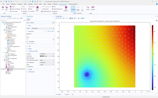
Note that only the load vector is modified. The other matrices and vectors are merely extracted and then put back into the system again.

This example is part of a collection available for download:

www.comsol.com/model/application-programming-guide-examples-140771

The relevant file for this example is:

•

accessing_system_matrices.mph