The Study node in the model tree contains one or more study steps, instructions that are used to set up solvers and solve for the dependent variables. The settings for the Study and the Solver Configurations nodes can be quite complicated. Consider the simplest case for which you just need to create a study, add a study step, and run it.

Building on the example from the previous sections regarding stationary heat transfer, add a Stationary study step.

The call to the method run automatically generates a solver sequence in a data structure model.sol and then runs the corresponding solver. The settings for the solver are automatically configured by the combination of physics interfaces you have chosen. You can manually change these settings, as shown later in this section. The data structure model.sol roughly corresponds to the contents of the Solver Configurations node under the Study node in the model tree.

All low-level solver settings are available in model.sol. The structure model.study is used as a high-level instruction indicating which settings should be created in model.sol when a new solver sequence is created.

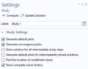
For backward compatibility, the low-level settings in model.sol can be automatically generated when using Record Code. This behavior is controlled by the Store complete solver history checkbox, available in the Settings window of the each Study node.

The example below shows a slightly more detailed approach to programming a study setup, based on the stationary heat transfer example shown earlier. These instructions more closely reflect the autogenerated output produced when Record Code is enabled and Store complete solver history is selected.

First, create instances of the Study node (with tag std1) and a Stationary study step subnode:

The actual settings that determine how the study is run are contained in a sequence of operations in the Solution data structure, with tag sol1, which is linked to the study:

The following code defines the sequence of operations contained in sol1.

First, create a Compile Equations node under the Solution node to determine which study and study step will be used:

Next, create a Dependent Variables node, which controls the scaling and initial values of the dependent variables and determines how to handle variables that are not solved for:

Now create a Stationary Solver node. The Stationary Solver contains the instructions that are used to solve the system of equations and compute the values of the dependent variables.

Add subnodes to the Stationary Solver node to choose specific solver types. In this example, use an Iterative solver:

Add a Multigrid preconditioner subnode:

You can have multiple Solution data structures in a study node (such as sol1, sol2, and so on) defining different sequences of operations. The process of notifying the study of which one to use is done by “attaching” the Solution data structure sol1 with study std1:

The attachment step determines which Solution data structure sequence of operations should be run when selecting Compute in the COMSOL Desktop user interface.

Finally, run the study, which is equivalent to running the Solution data structure sol1:

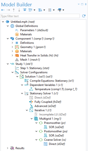
The resulting Study node structure is shown in the figure below. Note that there are several additional nodes added automatically. These are default nodes and you can edit each of these nodes by explicit method calls. You can edit any of the nodes while using Record Code to see the corresponding methods and syntax used.

where studyTag equals "std1", or similar, depending on the model’s configuration.

For example, in a model with a study that has the study tag std1, the corresponding code would be:

In a typical case, when Record Code or Record Method is enabled and Store complete solver history is disabled, the recorded code will appear as follows:

The line calling setSolveFor is used to specify whether a particular physics interface should be included in the computation. In this example, setSolveFor("/physics/ht", true) ensures that the Heat Transfer interface is enabled in the study.

To illustrate how some of the low-level solver settings can be modified, consider a case where the settings for the Fully Coupled node are modified. This subnode controls the type of nonlinear solver used.

The first line below may not be needed depending on whether the Fully Coupled subnode has already been generated or not (it could have been automatically generated by code similar to what was shown above).

For more information on the meaning of these and other low-level solver settings, see the Solver section of the Programming Reference Manual.

Changing the low-level solver settings requires that model.sol has first been created. It is always created the first time you compute a study, however, you can trigger the automatic generation of model.sol as follows:

where the call to showAutoSequences corresponds to the option Show Default Solver, which is available when right-clicking the Study node in the model tree.

This can be used if you do not want to take manual control over the settings in model.sol (the solver sequence) and are prepared to rely on the physics interfaces to generate the solver settings. If your application makes use of the automatically generated solver settings, then updates and improvements to the solvers in future versions are automatically included. Alternatively, the automatically generated model.sol can be useful as a starting point for your own edits to the low-level solver settings.

When creating an application it is often useful to keep track of whether a solution exists or not. The method model.sol("sol1").isEmpty() returns a boolean and is true if the solution structure sol1 is empty. Consider an application where the solution state is stored in a string solutionState. The following code sets the state depending on the output from the isEmpty method:

Alternatively, solutionState can be initialized to noSolution and the following code is used to indicate a state change corresponding to the input values having changed: