Distillation is the most prominent separation method in chemical process industries. In a typical application, as shown in Figure 12, a liquid mixture of two or more species is fed into a tall cylindrical column somewhere near the middle. For purpose of illustration, this example is limited to two species. There is a heat source in a collecting vessel or column section at the bottom of the column called the reboiler. Liquid from the feed runs down the column and is heated and partially vaporized in the reboiler. Normally, some of the liquid in the reboiler is continuously removed as the bottoms product. The vapor generated in the reboiler rises up toward the top of the column where it is condensed in an externally cooled vessel or column section called the condenser. Some of the condensed liquid in the condenser is normally removed as the overhead product or distillate. The remainder of the condensed liquid is sent back down the column as reflux. With heat added at the bottom and removed at the top, the temperature decreases from bottom to top of the column that operates at nearly constant pressure.
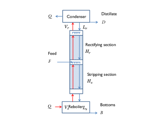
Here Ls is the liquid flow rate from the stripping section into the reboiler,
Lr is the liquid flow rate from the condenser into the rectifying section, and
F the feed flow rate. Other feed conditions would alter the analysis slightly since some or all of the feed would join the vapor phase in the rectifying section.
where xf,
xb, and
xd are mole fractions of the more volatile species in the feed, bottoms, and distillate streams, respectively.
along with Equation 6. All of these flow rates are found in the model by algebraic manipulation in the
Parameters node under
Global Definitions in the Model Builder.
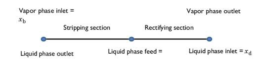
Neglecting any variation in the radial direction, model the distillation column in one dimension using two line segments (see Figure 13). One segment of length,
Hs, represents the stripping section, while the other segment of length
Hr, represents the rectifying section. The goal of the model is to determine the values of
Hs and
Hr that provide the specified bottoms and distillate compositions. Assume values of
Hs and
H =
Hs +
Hr, solve for the compositions in the vapor and liquid phases at every point in the column, and iterate until the outlet compositions match the design specifications.
where Kya is an overall gas phase mass transfer coefficient in mol/(m
3·s),
ye1 is the mole fraction of the more volatile species that would be reached at equilibrium, and
M1 is the molar mass of the more volatile species. This provides a mass transfer rate of the more volatile species from the liquid phase to the vapor phase. A similar expression with opposite sign describes the simultaneous mass transfer of the less volatile component in accordance with our constant molar overflow assumption. The value of
ye1 at each point is found using an Equilibrium Calculation node added in the Thermodynamic System under Thermodynamics. The mass transfer coefficient will depend on the fluid and packing properties and the local fluid velocities and may vary along the height of the column. Correlations for
Kya are available in the literature. In this example, a constant value of
Kya = 75 mol/(m
3·s) is used for illustrative purposes.
The boundary conditions for this mass transfer problem are shown in Figure 13. You specify the mass fraction of the bottoms in the vapor phase and the mass fraction of the feed and distillate in the liquid phase.
Hs and
H are varied by guess and check or using a parameter sweep until a solution is found where the liquid phase bottoms composition equals that specified in the vapor phase, and the vapor phase distillate composition equals that specified in the liquid phase.
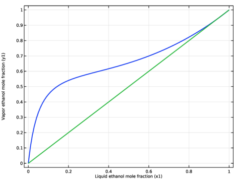
Figure 14 shows the results of an equilibrium calculation, available in Thermodynamics, generating an
xy diagram for the ethanol–water system at 1 atm pressure. The NRTL thermodynamic model is used for the liquid phase, while an ideal gas assumption is used for the gas phase.
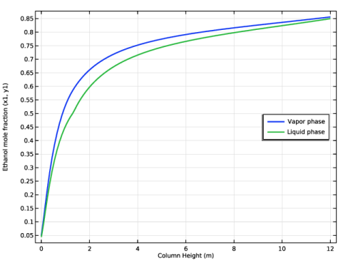
The calculated results for vapor and liquid phase compositions inside a column designed to separate a 50 mole percent mixture of ethanol in water to yield a distillate of 85 mole percent ethanol and a bottoms product of 5 mole percent ethanol are shown in Figure 15. The required heights found by trial are
Hs = 1.2 m and
H = 5.7 m. In the model a Parametric Sweep study step was used to compute the column composition when varying the stripping section length. The design criteria to be met in this case is that the ethanol mole fraction in the vapor and liquid phase should coincide at the bottom. Using a section length less than about 1.2 m, the liquid phase mole fraction exiting the column is higher than that of the vapor phase. Correspondingly, for a section longer than 1.2 m, the liquid phase mole fraction is lower than that of the vapor phase. The same analysis can be made for the top of the column. The optimal column height is found when the phase compositions match also at the top.
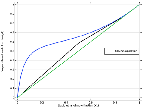
Figure 16 presents the results from
Figure 15 on an
xy plot along with the equilibrium curve of
Figure 14. Readers familiar with the traditional McCabe–Thiele distillation analysis will note that it is no coincidence that our calculated results trace out straight operating lines for the stripping and rectifying sections that intersect at the feed composition for this case with a saturated liquid feed.