|
1
|
|
2
|
In the Settings window for 1D Plot Group, type Density in the Label field.
|
|
5
|
In the Settings window for Global, locate the y-Axis Data section. Click Replace Expression
|
|
6
|
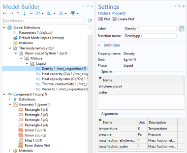
In the table, enter the following arguments for the function: Tc, pRef, w_EG, w_W. Make sure to add the arguments in this order. This is the order defined in the Mixture node.
|
|
3
|
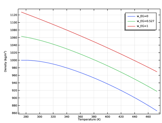
Select the x-axis label checkbox and type Temperature (K).
|
|
4
|
Select the y-axis label checkbox and type Density (kg/m<sup>3</sup>).
|
|
2
|
In the Settings window for 1D Plot Group, type Viscosity in the Label field.
|
|
5
|
In the Settings window for Global, locate the y-Axis Data section. Click Replace Expression
|
|
3
|
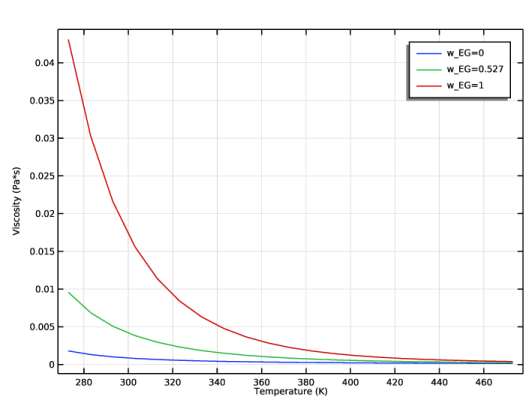
Select the x-axis label checkbox and type Temperature (K).
|
|
4
|
Select the y-axis label checkbox and type Viscosity (Pa\cdot s).
|
|
2
|
In the Settings window for 1D Plot Group, type Thermal Conductivity in the Label field.
|
|
5
|
In the Settings window for Global, locate the y-Axis Data section. Click Replace Expression
|
|
3
|
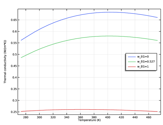
Select the x-axis label checkbox and type Temperature (K).
|
|
4
|
Select the y-axis label checkbox and type Thermal conductivity (W/(m\cdot K)).
|
|
2
|
In the Settings window for 1D Plot Group, type Heat Capacity in the Label field.
|
|
5
|
In the Settings window for Global, locate the y-Axis Data section. Click Replace Expression
|
|
3
|
Select the x-axis label checkbox and type Temperature (K).
|
|
4
|
Select the y-axis label checkbox and type Heat capacity (J/(kg\cdot K)).
|