Engine Coolant Properties
Introduction
The engine block of a car includes a cooling jacket to remove excess heat from combustion. The cooling jacket consists of open spaces in the cylinder block and the cylinder head. When the engine is running, a coolant fluid is pumped through the jacket to keep the engine from overheating. Optimizing the heat removal is important to minimize coolant boiling, prevent engine failure, and, more recently, improve overall efficiency through waste heat recovery. This example demonstrates how the Thermodynamics feature can be used to evaluate the performance of different engine coolants.
Although pure water works well as a coolant, to prevent freezing at low temperatures, a mixture of ethylene glycol and water is normally used to lower the freezing point. The Thermodynamics feature is used here to show how the boiling point, density, viscosity, thermal conductivity, and heat capacity also depend on the composition of the coolant mixture and how changes in these properties affect the cooling process.
Model Definition
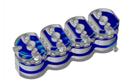
Figure 4 shows the flow pattern inside the cooling jacket of a representative four cylinder engine. Solving a fully coupled nonisothermal turbulent flow problem with temperature-, pressure-, and composition-dependent coolant properties in this complex geometry typically requires a significant number of computer hours. One approach to obtain a reliable approximate solution in a shorter time is to use the functionality available in the Thermodynamics feature to investigate the coolant property behavior and determine where simplifying assumptions can be made. The consequences of these assumptions can be investigated efficiently in a simplified geometry in order to provide confidence in their use in more complex geometries.
Figure 4: The coolant flow inside the coolant jacket of a four-cylinder engine.
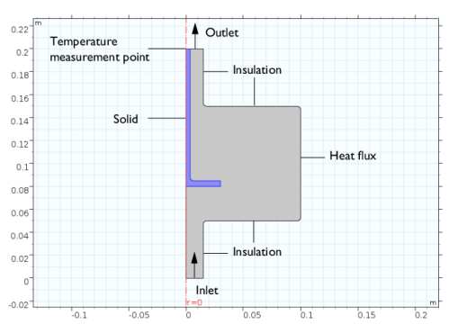
Here, a simplified 2D axially symmetric geometry, shown in Figure 5, is considered as an engine coolant test apparatus. Coolant is introduced at a specified flow rate in the bottom of the device, the coolant hits a solid steel part and is then deflected into a larger flow domain. A heat flux is applied on the outer boundary of the larger section. The resulting temperature is measured at steady state in the solid structure near the coolant outflow at the top.
To solve for the fluid flow and heat transfer in the test apparatus, the current model uses the Single-Phase Flow and the Heat Transfer in Fluids interfaces. The interfaces are coupled using a Nonisothermal Flow multiphysics feature, and the k-ε model is used to model the fluid flow turbulence.
The properties of the coolant fluid are defined using the Thermodynamics feature. This is done by first defining and adding a Thermodynamic System node to the Thermodynamics feature. Included in the Thermodynamic System are the relevant chemical species, in this case ethylene glycol and water. The Thermodynamic system node in turn can be used to compute property functions for thermodynamic properties and transport properties, both for the pure species and for the resulting mixture. In this case, functions for the density, the viscosity, the thermal conductivity and the heat capacity of the coolant mixture are created.
The analysis of the coolant properties is performed in three steps. First, the mixture properties are evaluated by plotting the functions created by the Thermodynamic System. Then the phase envelope of the coolant vapor-liquid system is visualized by plotting the equilibrium temperatures (for boiling and condensation) as a function of the composition. The required equilibrium functions are defined by adding an Equilibrium Calculation feature to the Thermodynamic System. Using the equilibrium functions the phase envelope for two different pressures are compared.
The fluid flow and heat transfer of the coolant mixture inside the test apparatus are then solved for. Results for pure water, and a 50 volume percent mixture of ethylene glycol in water are compared. For these chemicals, a 50 volume percent mixture corresponds to 52.7 mass percent of ethylene glycol. Finally the results are used to compute average mixture properties.
Figure 5: Axially symmetric engine coolant test apparatus.
Results
Figure 6 shows the temperature and composition dependence of the heat capacity. Similar graphs are generated for density, viscosity, and thermal conductivity. Studying these graphs reveals that the addition of ethylene glycol increases the density and viscosity, but decreases the thermal conductivity and heat capacity when compared with pure water. It should be expected that a 50 volume percent mixture will yield a higher pressure drop and require a higher flow rate to achieve the same cooling effect as that of pure water.
Figure 6: Heat capacity as a function of temperature and composition for ethylene glycol water mixtures.
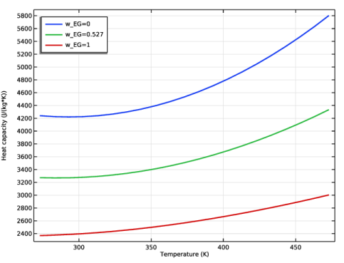
Figure 7 shows the phase envelope for ethylene glycol-water mixtures produced using the Equilibrium Calculation feature of the Thermodynamic System. A car coolant system typically operates at about 2 atm pressure. Here we can see that a 50 volume percent (24.4 mole percent) mixture should boil at a temperature slightly above than 400 K at this pressure.
Figure 7: Phase envelope for the equilibrium temperature of ethylene glycol-water mixtures at two pressures.
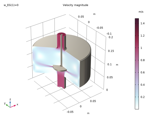
Figure 8 shows the flow pattern inside the test apparatus with water entering at 1 m/s. The coolant flow of 42 l/min and a heat input of 50 kW used here in the test apparatus are on the same order of magnitude as in a conventional car cooling system.
Figure 8: Flow patterns inside the test apparatus with water at 1 m/s.
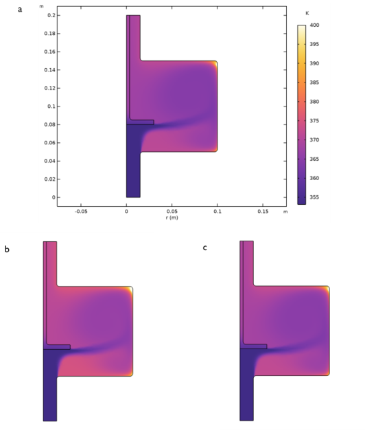
As expected, Figure 9 shows that an ethylene glycol-water mixture will provide less cooling than pure water at a fixed flow rate. About 15 percent more coolant flow is required to produce the same cooling as when using pure water. It can also be seen that some boiling of the coolant (at T > 400 K) is expected in the recirculation zones in the outer corners of the apparatus.
Figure 9: Temperature within the test apparatus for three cases: (a) water at 1 m/s, (b) 50 volume percent ethylene glycol at 1 m/s, and (c) 50 volume percent ethylene glycol at 1.15 m/s.
The table below provides a comparison of results for pressure drop, outlet temperature, and outlet density.
1 Using constant mixture properties.
Considering the graphical results for the various coolant properties, it might be best to use approximate averages for the relatively small temperature range of 353–400 K. In Figure 10 the resulting heat capacities for the pure water and the two ethylene glycol-water mixture cases are plotted. As seen before, the heat capacity differs significantly when comparing pure water and the mixture. But, the individual variation for each coolant however is seen to be small, about 2% for this mixture property and location. Analyzing the density in the same manner, the variation can be seen to be in the same order of magnitude.
Figure 10: Coolant heat capacity plotted along a vertical cut line at half the radius of the test apparatus chamber.
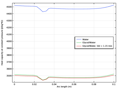
Using the solution for a mixture with 50 volume percent ethylene glycol in water, the following average values are computed: density = 1010 kg/m3, viscosity = 9.07·10-4 Pa·s, thermal conductivity = 0.574 W/(m·K), and heat capacity = 3486 J/(kg·K). 
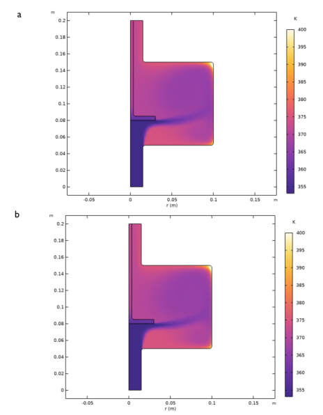
Figure 11 shows a comparison of the temperature results obtained using these approximations with those using the fully coupled temperature-dependent properties in our test device. The similarity between these results is sufficient to justify the use of the approximate average values in a cooling jacket model with a realistic geometry. Solving the flow and heat transfer equations requires considerably less computational effort for the constant average property value case.
Figure 11: Comparison of temperature within our test apparatus for 50 volume percent ethylene glycol in water at 1 m/s using: (a) temperature dependent properties, (b) approximate average properties.
Reference
1. http://www.engineeringtoolbox.com/ethylene-glycol-d_146.html
Modeling Instructions: Engine Coolant Properties
The following step-by-step instructions guide you through the process of setting up a Thermodynamic System, build a geometry, and simulate the engine coolant physics using the Single Phase Flow, and Heat Transfer in Fluids interfaces. The Thermodynamic System is created from the COMSOL thermodynamic database, which provides all necessary thermodynamic and transport properties.