Introduction
The CFD Module is used by engineers and scientists to understand, predict, and design for fluid flow in closed and open systems. At a given cost, these types of simulations typically lead to new and better products and improved operations of devices and processes compared to purely empirical studies involving fluid flow. As part of an investigation, simulations give accurate estimates of flow patterns, pressure losses, forces on submerged objects, temperature distributions, and variations in fluid composition within a system.
Figure 1: Streamlines and free-surface deformation for the flow around a torpedo.
The CFD Module’s general capabilities include modeling stationary and time-dependent fluid flow problems in two- and three-dimensional spaces. Formulations for different types of flow are predefined in a number of Fluid Flow interfaces, which allow you to set up and solve a variety of fluid-flow problems. These physics interfaces define a fluid-flow problem using physical quantities, such as velocity and pressure, and physical properties, such as viscosity. The Fluid Flow interfaces cover a wide range of flows, such as laminar and turbulent single-phase, multiphase, nonisothermal, and reacting flows.
The physics interfaces build on conservation laws for momentum, mass, and energy. These laws are expressed in terms of partial differential equations, which are solved by the module together with the specified initial and boundary conditions. The equations are solved using stabilized finite element formulations for fluid flow in combination with damped Newton methods and, for time-dependent problems, different time-dependent solver algorithms. The results are presented in the Graphics window through predefined plots relevant for CFD, expressions of physical quantities that you can freely define, and tabulated derived quantities (for example, average pressure on a surface or drag coefficients) obtained from a simulation.
The workflow in the CFD Module is quite straightforward and is described by the following steps: define the geometry, select the fluid to be modeled, select the type of flow, define boundary and initial conditions, define the finite element mesh, select a solver, and visualize the results. All these steps are accessed from the COMSOL Desktop®. The mesh and solver steps are usually carried out automatically using default settings that are tuned for each specific Fluid Flow interface.
The CFD Module Application Library describes the Fluid Flow interfaces and their different features through tutorial and benchmark examples for the different types of flow. Here you can find models of industrial equipment and devices, tutorials for practice, and benchmark applications for verification and validation of the Fluid Flow interfaces.
This introduction is intended to give you an accelerated start in CFD application building. It contains examples of the typical use of the module, a list of all the Fluid Flow interfaces including a short description of each, and two tutorial models, Tutorial Model — Backstep and Tutorial Model — Water Purification Reactor, to introduce the workflow.
Aspects of CFD Simulations
The physical nature of a flow field may be characterized by a set of dimensionless numbers such as the Reynolds number, the Mach number, and the Grashof number. A great deal of information about the flow field can be gained by analyzing these numbers.
The Reynolds number, for example, expresses the ratio of the inertia forces to the viscous (internal friction) forces. For vanishingly small values of the Reynolds number, the inertia forces are negligible and the flow is reversible, in the sense that reversed boundary conditions lead to reversed flow. The energy dissipation is immediate. As the Reynolds number increases, viscous effects become more and more confined to boundaries, internal shear layers, and wakes. The relative size and other characteristics of such regions are determined by the Reynolds number. Eventually, for very large values of the Reynolds number, the flow becomes fully turbulent. In contrast to laminar flow at high Reynolds numbers, viscous dissipation is active everywhere in a turbulent flow field but is most effective on the smallest flow structures. The energy is transferred from the large-scale flow structures to the small-scale flow structures through a cascade of eddies. Due to the requirement of resolving all these flow scales, direct numerical simulation of industrially relevant turbulent flows is currently not a feasible approach. Instead, turbulence models are applied when analyzing these flows. For very small values of the Reynolds number, the CFD Module offers the Creeping Flow interface; for intermediate values, the Laminar Flow interface; and for large values, the Turbulent Flow, Large Eddy Simulation, and Detached Eddy Simulation interfaces.
You can use the Two-Phase Flow and Three-Phase Flow interfaces in the Multiphase Flow branch to model moving, deformable interfaces between phases, separating two or three different fluids. The other physics interfaces in this branch are mainly intended for modeling suspensions of many particles, droplets, or bubbles. Among the latter group, the Euler–Euler Model interface is able to handle high concentration levels with frequent collisions as well as transients in the relative velocity between the phases (that is, nonvanishing ratios of the particle relaxation time to the macroscopic flow time scale). The Phase Transport, Mixture Model physics interface can be used to model transport of multiple dispersed phases.
Temperature variations caused by heat transfer, compression work, or work done by friction forces result in an inhomogeneous density field which may trigger thermal convection. The significance of thermally induced buoyancy forces in the momentum equation is characterized by the ratio of the Grashof number to the square of the Reynolds number (for large Reynolds numbers), or of the Grashof number to the Reynolds number (for small Reynolds numbers). For nonvanishing values of this ratio, the Nonisothermal Flow interfaces are available.
The Mach number expresses the ratio of the speed of the fluid to the speed of sound of the flowing medium. This dimensionless number measures the relevance of compressible effects in the flow field, predicting occurrences of shock waves and rarefaction waves. For Mach numbers greater than 0.3, the laminar, turbulent, and Euler equations versions of the High Mach Number Flow interfaces are available.
The Shallow Water Equations interface and the Thin-Film Flow interfaces provide simplified, depth-averaged formulations for free-surface flows and lubrication applications, respectively.
For reacting flow and flow in porous media, the Chemical Species Transport branch and the Porous Media and Subsurface Flow branch are available.
Contrary to experimental analyses, which are most often performed in a laboratory where measurements are limited to a small number of points, a CFD simulation gives a “big picture” view of the flow field. A qualitative interpretation of the flow and pressure fields is usually the first step toward creating or improving a design.
Figure 2 shows the flow field around a solar panel. The presence of a wake in front of the panel, caused by another panel in the solar power plant, may induce lift forces that would not be present if the panel were analyzed alone. Three-dimensional graphics such as surface, streamline, ribbon, arrow, and particle-tracing plots, as well as animations that include any combination of the aforementioned features, are examples of tools you can use for qualitative studies.
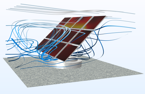
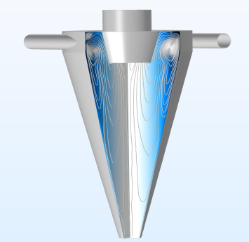
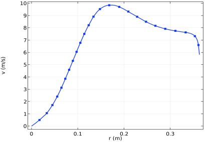
Figure 2: Turbulent fluid flow around a solar panel solved using the CFD Module.
In addition to the qualitative “big picture” view, simulations performed with the CFD Module give accurate quantitative estimates of properties of the flow field, such as the average flow at a given pressure difference, the drag and lift coefficients around submerged bodies, or the air quality in a ventilated room.
Figure 3 and Figure 4 show the velocity and pressure fields in a cyclone simulation. The centrifugal force, which is proportional to the square of the azimuthal velocity component and the inverse of the radius, can be used to assess the separation efficiency in the cyclone. In addition to separation and fractionation, cyclones may be used for deflocculation, which can be modeled using the turbulent dissipation rate.
Figure 3: In-plane streamlines and pressure field for the flow field in a cyclone simulated using the v2-f turbulence model.
Figure 4: Azimuthal velocity component below the vortex finder. The characteristic profile due to a free vortex can be observed for larger radii.
The CFD Module has a vast range of tools for evaluating quantitative results. For example, it comes with built-in functionality for evaluating surface and volume averages, maximum and minimum values, and derived values (functions and expressions of the solution), as well as for generating tables and xy plots. Derived values such as drag and lift coefficients and other values relevant for CFD are easily defined.
Qualitative studies typically form the basis for understanding, which in turn can spark new ideas. These ideas can then lead to significant improvements to products and processes, often in quantum leaps. Quantitative studies, on the other hand, form the basis for optimization and control, which can also greatly improve products and processes but usually do so through a series of many smaller steps.