The Periodic Port is a dedicated feature used to model transmission, reflection, and scattering problems for periodic structures such as, for example, absorbers and diffusers. The feature is in particular interesting for diffusers as it can split the reflected energy into specular an non-specular directions. The periodic port handles plane wave incidence on the structures as well as all reflected and transmitted diffraction orders (when set up). The condition exists in 3D and 2D. The
Periodic Port condition is set up together with a
Periodic Condition with the
Floquet periodicity (Bloch periodicity) option.
This section is present if Incident wave excitation at this port is set to
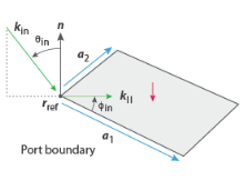
On and the model is 3D. Select the reference corner used to define a local coordinate system at the port surface for defining the incident wave direction (see details below).
Activate if the given port is excited by an incident plane wave. For the first Periodic Port condition added in a model, the
Incident wave excitation at this port is set to
On. For subsequent conditions added, the excitation is set to
Off per default.
When the Incident wave excitation at this port is set to
On, then select how to define the incident plane wave. Set
Define incident wave to
Amplitude (the default) or
Power.
For both options, enter the phase φ (SI unit: rad) of the incident wave. This phase contribution is multiplied with the amplitude defined by the above options. The
Amplitude input can be a complex number.
In 2D enter the Polar angle of incidence ϕin. In 3D models enter both the
Polar angle of incidence ϕin and the
Azimuthal angle θin.
When the Incident wave excitation at this port is set to
Off, then select the incident port in the
Mode settings from incident periodic port combo (default is
Not defined). This ensures that the orientation of the local coordinate systems on the two periodic ports are consistent.
To display this section, click the Show More Options button (

) and select
Advanced Physics Options in the
Show More Options dialog. For information about the
Constraint Settings section, see
Constraint Settings in the
COMSOL Multiphysics Reference Manual.