|
•
|
Pressure acoustics: model the propagation of sound waves (pressure waves) in the frequency domain solving the Helmholtz equation or in the time domain solving the scalar wave equation. Pressure acoustics comes in different flavors depending on the numerical formulation used. This includes finite element (FEM) based interfaces for frequency and transient models, a boundary element (BEM) based interface only used in the frequency domain, and a discontinuous Galerkin (dG-FEM) formulation based interface used for transient simulations. The Acoustics Module has built-in couplings between BEM and FEM that allows for modeling hybrid FEM-BEM problems.
|
|
•
|
Acoustic-structure interaction: combine pressure waves in the fluid with elastic waves in the solid to model vibroacoustic problems. The physics interfaces provide predefined multiphysics couplings at the fluid-solid interface.
|
|
•
|
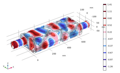
Boundary mode acoustics: find propagating and evanescent modes in ducts and waveguides. The analysis exists for classical pressure acoustic, elastic waves, thermoviscous acoustics, and convected acoustic problems.
|
|
•
|
Thermoviscous acoustics: model the detailed propagation of sound in geometries with small length scales. This is acoustics including thermal and viscous losses explicitly. Also known as microacoustics, viscothermal acoustics, or linearized compressible Navier–Stokes. In the time domain, nonlinear effects can be included.
|
|
•
|
Aeroacoustics: model the influence a background mean flow has on the propagation of sound waves in the flow, so-called, convected acoustics or flow borne noise/sound. Interfaces exist to solve the linearized potential flow, the linearized Euler equations, and the linearized Navier–Stokes equations in both time and frequency domain.
|
|
•
|
Flow-induced noise: model the noise generated by a turbulent flow using the Lighthill analogy to set up an aeroacoustic flow source in pressure acoustics.
|
|
•
|
Compressible potential flow: determine the flow of a compressible, irrotational, and inviscid fluid.
|
|
•
|
Solid mechanics and elastic waves: solve structural mechanics problems and the propagation of elastic waves in solids.
|
|
•
|
Piezoelectricity: model the behavior of piezoelectric materials in a multiphysics environment solving for the electric field and the coupling to the solid structure.
|
|
•
|
Poroelastic waves: in porous materials model the coupled propagation of elastic waves in the solid porous matrix and the pressure waves in the saturation fluid. Biot’s equations are solved here. Includes options to include both thermal and viscous losses.
|
|
•
|
Ultrasound: in ultrasound problems transient propagation is important and it is also important to be able to solve models with many wavelengths. These interfaces are based in the discontinuous Galerkin or dG-FEM formulation.
|
|
•
|
Nonlinear acoustics: model nonlinear acoustic phenomena like the cumulative nonlinear effects by solving the Westervelt equation. Local nonlinear effects such as vortex shedding can be included using the nonlinear thermoviscous acoustic functionality.
|
|
•
|
Acoustic diffusion equation: solve a diffusion equation for the acoustic energy density distribution for systems of coupled rooms in room acoustic applications.
|
|
•
|
Ray acoustics: compute trajectories and intensity of acoustic rays in room acoustic as well as underwater acoustic applications. Determine the impulse response and room acoustic metrics with dedicated features in postprocessing.
|
|
•
|
Pipe acoustics: use this physics interface to model the propagation of sound waves in pipe systems including the elastic properties of the pipe. The equations are formulated in 1D for fast computation and can include a stationary background flow.
|
|
•
|
Acoustic streaming: use these multiphysics capabilities to couple pressure acoustics or thermoviscous acoustics to a fluid flow interface to model acoustic streaming, that is flow induced by sound.
|