Results
You chose not to have new default plots generated. Once the solution process is finished you can use the existing plot groups and just switch the dataset to see how the damping material affects the solution.
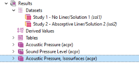
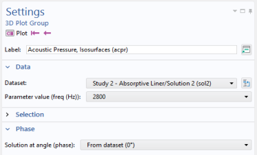
Acoustic Pressure, Isosurfaces (acpr)
1
In the Model Builder under Results, click the Acoustic Pressure, Isosurfaces (acpr)
node.
2
In the Settings window for 3D Plot Group under Data, from the Dataset list choose Study2/Solution 2.
3
In the Settings window click the Plot button
.
At 2800 Hz, the pressure in the chamber is much lower than before.
Proceed to study how the transmission loss has changed with the addition of the lining. Duplicate the first plot and select the new dataset, first do a bit of formatting.
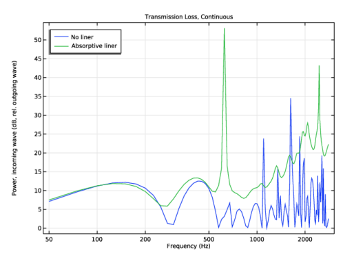
Transmission Loss, Continuous
1
In the Model Builder window, under Results click Transmission Loss, Continuous.
2
In the Settings window for 1D Plot Group, click to expand the Title section.
3
From the Title type list, choose Manual.
4
In the Title text area, type Transmission Loss, Continuous.
5
Locate the Plot Settings section. Select the y-axis label checkbox.
6
In the associated text field, type Power, incoming wave (dB, rel. outgoing wave).
7
Click to expand the Legend section. From the Position list, choose Upper left.
8
In the Model Builder window, under Results > Transmission Loss, Continuous right-click Octave Band Plot 1 and choose Duplicate.
9
In the Settings window for Octave Band Plot, locate the Data section.
10
From the Dataset list, choose Study 2/Solution 2 (sol2).
11
Click to expand the Legends section. In the table, enter the following settings:
Legends
Absorptive liner
12
On the Transmission Loss, Continuous toolbar, click Plot
.
The plot should look like that in
Figure 12
top.
Duplicate the Transmission Loss plot and change the format to 1/3 octave bands.
Transmission Loss, Continuous 1
1
In the Model Builder window, right-click Transmission Loss, Continuous and choose Duplicate.
2
In the Settings window for 1D Plot Group, type Transmission Loss, 1/3 Octave Bands in the Label text field.
3
Locate the Title section. In the Title text area, type Transmission Loss, 1/3 Octave Bands.
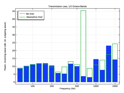
Transmission Loss, 1/3 Octave Bands
1
In the Model Builder window, expand the Results > Transmission Loss, 1/3 Octave Bands node, then click Octave Band Plot 1.
2
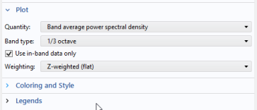
In the Settings window for Octave Band Plot, locate the Plot section.
3
From th Quantity list, choose Band average power spectral density
4
From the Band type list, choose 1/3 octave bands.
5
In the Model Builder window, under Results > Transmission Loss, 1/3 Octave Bands click Octave Band Plot 2.
6
In the Settings window for Octave Band Plot, locate the Plot section.
7
From the now Band type list, choose 1/3 octave bands.
8
Locate the Coloring and Style section, then click to expand the Coloring and style section. From the Type list, choose Outline.
9
In the Width text field, type 2.
10
On the Transmission Loss, 1/3 Octave Bands toolbar, click Plot
.
The plot should look like that in
Figure 12
bottom.
Now, create a plot that represents the intensity flux through the muffler system. Use streamlines that follow the intensity vector (flux of energy through the muffler). You can change between solutions and frequencies to study and visualize the muffler’s sound-absorbing properties.
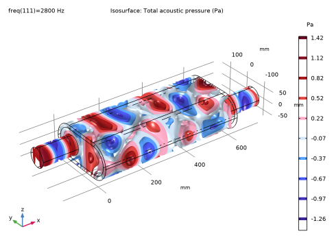 At 2800 Hz, the pressure in the chamber is much lower than before.