Results
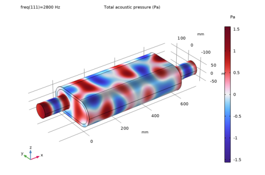
The first default plot shows the pressure distribution on the walls of the muffler at the highest frequency, 2800 Hz.
Acoustic Pressure (acpr)
The pattern is very different at different frequencies. See for example what happens at 1250 Hz.
1
In the Model Builder under Results, click Acoustic Pressure (acpr)
.
2
Go to the Settings window for 3D Plot Group. Under Data from the Parameter value (freq) list, choose 1250.0.
3
On the 3D Plot Group toolbar click the Plot button
.
At 1250 Hz, the absolute value of the pressure does not vary much with the x-coordinate. The reason is that this is just higher than the cutoff frequency for the first symmetric propagating mode, which is excited by the incoming wave. For a separate analysis of the propagating modes in the chamber, see the description for the
Eigenmodes in a Muffler
model.
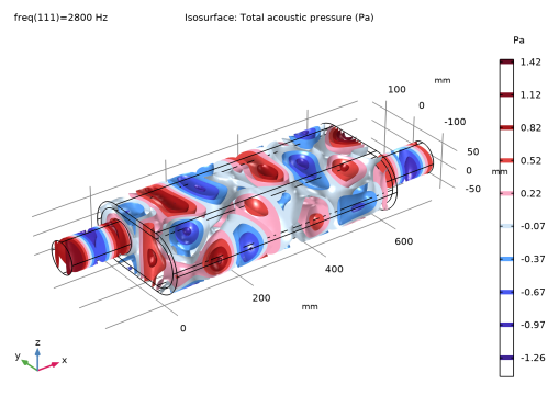
The two other default plot groups show the sound pressure level on the wall surface and the pressure inside the muffler as isosurfaces.
Acoustic Pressure, Isosurfaces (acpr)
1
In the Model Builder under Acoustic Pressure, Isosurfaces (acpr), click the Isosurface node
to display the plot in the next figure.
Proceed to plot the transmission loss of the muffler system. Use the Octave Band Plot as it allows to plot any transfer function both as band plots and as continuous curves (sweeps).
1D Plot Group 4
1
In the Home toolbar, click Add Plot Group and choose 1D Plot Group
.
2
In the Settings window for 1D Plot Group, type Transmission Loss, Continuous in the Label text field.
Transmission Loss, Continuous
1
On the Transmission Loss, Continuous toolbar, select Octave Band under More plots, click Octave Band Plot
.
2
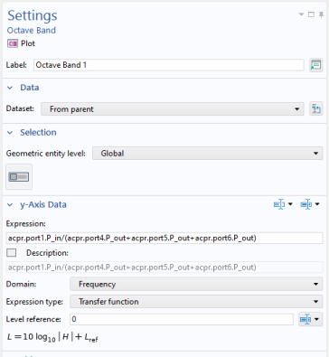
In the Settings window for Octave Band Plot, locate the Selection section.
3
From the Geometric entity level list, choose Global.
Start by locating and inspecting the postprocessing variables available for the port boundary conditions. Add the variable for the power of the incident mode at Port 1. Then modify the expression manually to get the ratio to the power of all the outgoing modes at Port 4, 5, and 6. This will give the transmission loss.
4
In the upper-right corner of the y-axis data section, click Replace Expression
. From the menu, choose Component 1 > Pressure Acoustics, Frequency Domain > Ports > Port 1 > acpr.port1.P_in - Power of incident mode - W.
5
Locate the y-Axis Data section. In the Expression text field, type acpr.port1.P_in/(acpr.port4.P_out+acpr.port5.P_out+acpr.port6.P_out).
6
From the Expression type list, choose Transfer function.
7
Locate the Plot section. From the Style list, choose Continuous.
8
Locate the Legends section. Select the Show legends checkbox.
9
From the Legends list, choose Manual.
10
In the table, enter the following settings:
Legends
No liner
11
On the Transmission Loss, Continuous toolbar, click Plot
.
The plot should be a reproduction of the blue curve in
Figure 12
.