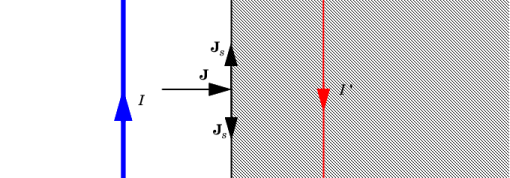
The Impedance Boundary Condition provides a boundary condition that is useful at exterior boundaries, where the electromagnetic field penetrates only a short distance outside the boundary. The boundary condition approximates this penetration to avoid the need to include another domain in the model. The material properties that appear in the equation are those for the conductive material excluded from the model.

The impedance boundary condition is a valid approximation if the skin depth is small compared to the size of the conductor. The source electric field Es can be used to specify an additional source surface current on the boundary.

where n is an outer normal. In frequency domain, the surface current can be related to the tangential electric field using the following admittance form:

where ω = 2πf, and

The skin depth (that is, the distance where the electromagnetic field has decreased by a factor e−1) can be computed as

where the skin depth is computed at a certain reference frequency ωc. The surface current is computed then as

The Harmonic Perturbation subnode (it is of the exclusive type) is available from the context menu (right-click the parent node) or in the Physics toolbar, click the Attributes menu and select Harmonic Perturbation. You can use it to specify a perturbation source electric field Es. For more information see Harmonic Perturbation — Exclusive and Contributing Nodes in the COMSOL Multiphysics Reference Manual.

The following material properties can be defined for the domain outside the boundary, which this boundary condition approximates. The default use the values From material. For User defined enter different values or expressions.

Based on space dimension, enter coordinate values or expressions for the Source electric field Es (SI unit: V/m).

For Frequency range, you can specify either Bandwidth and center (default) or Minimum and maximum.

In both cases, you can specify the approximation Accuracy. Note that both higher accuracy and wider frequency range can require using more auxiliary variables together with the corresponding ODEs to be solved during time domain and eigenfrequency computations.

The approximation computation needs to be done as a preprocessing step. Use the Compute approximation () action button available in the upper-right corner of Time Domain and Eigenfrequency section. The approximation computation is quick, and it will also compute and show the skin depth value at the center frequency. Once the computation has been performed, you can preview it using the Preview plot () action button that will become active at the section. You can also check the Show approximation data checkbox to inspect the actual computed values.