The AC/DC Module Physics Interfaces
The AC/DC interfaces are based on Maxwell’s equations, or subsets and special cases of these, together with material models. Different subsets of Maxwell’s equations in combination with special material models result in different electric, magnetic, or electromagnetic formulations. In the module, these laws of physics are translated by the AC/DC interfaces to sets of partial differential equations or integral equations with corresponding initial and boundary conditions.
An AC/DC interface defines a number of features. Each feature represents a term or condition in the underlying Maxwell-based formulation and may be defined in a geometric entity of the model, such as a domain, boundary, edge (for 3D components), or point.
Figure 5 on the next page shows the Model Builder window and the Settings window for the selected Charge Conservation in Solids 1 feature node in the Electrostatics interface. The Charge Conservation in Solids 1 node adds the terms representing Electrostatics to the model equations for a selected geometrical domain in the model.
Furthermore, the Charge Conservation in Solids 1 node may link to the Materials node to obtain physical properties, in this case the relative permittivity of a user-defined dielectric. The properties, defined by the Dielectric material node, may be functions of the modeled physical quantities, such as temperature. The Zero Charge 1 boundary condition feature adds the natural boundary conditions that limit the Electrostatics domain.
Figure 5: The Model Builder window (to the left), and the Settings window for Charge Conservation in Solids 1 for the selected feature node (to the right). The Equation section in the Settings window shows the model equations and the terms added to the model equations by the Charge Conservation in Solids 1 node. The added terms are underlined with a dotted line. The text also explains the link between the material properties represented by the Dielectric node and the values for the Relative permittivity.
The AC/DC Module has several AC/DC interfaces () for different types of electric and magnetic modeling. Figure 6 shows the AC/DC interfaces as well as predefined multiphysics combinations of more than one physics interface, some of which require additional licenses. Also see Physics Interface Guide by Space Dimension and Study Type.
Figure 6: The AC/DC Module physics interfaces as displayed in the Model Wizard for a 3D Space Dimension. The left column lists all physics interfaces under the AC/DC branch, some of which requires additional licenses such as the Structural Mechanics Module. The right column displays the available physics interfaces with the AC/DC Module license only.
As shown in Figure 6, the physics interfaces available under the AC/DC branch are categorized into different subbranches. A brief overview of different branches and physics interfaces follows.
Electric Fields and Currents
The Electric Fields and Currents branch () contains physics interfaces for analyzing electric fields, electric potential distributions, charge densities and current conservation at relatively low frequencies. Inductive effects are negligible; that is, the skin depth and wavelength are considered to be much larger than the studied device.
The Electrostatics interface () solves a charge conservation equation for the electric potential given the spatial distribution of the electric charge. It is used primarily to model charge conservation in dielectrics under static conditions. This physics interface applies also under transient conditions but then it is usually combined with a separate transport model for single species or multispecies charge transport. Such transport models can be found in the Chemical Reaction Engineering Module and in the Plasma Module. Some typical applications that are simulated in the Electrostatics interface are capacitors, dielectric sensors, and bushings for high voltage DC insulation.
The Electrostatics, Boundary Elements interface (), solves Laplace’s equation for the scalar electric potential. It is used for computing the potential distribution in dielectrics with constant and isotropic electric permittivity under conditions where the electric potential distribution on the boundaries is explicitly prescribed. The formulation is based on the boundary element method and the interface is available in 2D and 3D. It can be coupled to the Electrostatics interface to combine the modeling of large open regions (using the boundary element method) and the modeling of complex inhomogeneous and anisotropic dielectrics (using the finite element method).
The Electric Currents interface () is used to model DC, AC, and transient electric current flow in conductive and capacitive media. This physics interface solves a current conservation equation for the electric potential. Some examples of its use are designing busbars for DC current distribution and designing AC capacitors.
The Electric Currents in Shells interface () is available in 3D geometries. It applies to faces in 3D where it is used to model DC electric current flow confined to thin current-conducting shells of fixed or varying thickness. This physics interface solves a boundary current conservation equation for the electric potential. Modeling ground return current flow in the hull of a ship or in the body of a car are examples of simulations that can be done with this physics interface. It is the same interface as the Electric Currents in Layered Shells interface but with different settings (for single shell).
The Electric Currents in Layered Shells interface () is available in 3D geometries. It applies to faces in 3D where it is used to model DC electric current flow confined to thin current-conducting layered shells of fixed or varying thickness. This physics interface solves a boundary current conservation equation for the electric potential. It is the same interface as the Electric Currents in Shells interface but with different settings (for layered shells).
Magnetic Fields, No Currents
The Magnetic Fields, No Currents branch () contains physics interfaces for analyzing magnetostatic fields from permanent magnets and other current free magnetic sources. The formulation used in the contained interfaces is stationary, but for use together with other physics, time-domain modeling is also supported in 2D and 3D.
The Magnetic Fields, No Currents interface () is used to efficiently model magnetostatics in current free regions, for example, when designing permanent magnet-based devices. It solves a magnetic flux conservation equation for the magnetic scalar potential. This physics interface supports both linear media, media with magnetic saturation and time‑domain hysteresis.
The Magnetic Fields, No Currents, Boundary Elements interface (), solves Laplace’s equation for the scalar magnetic potential. It is used to compute magnetostatic fields from permanent magnets and other current free magnetic sources in media with constant and isotropic magnetic permeability. The formulation is based on the boundary element method and the interface is available in 2D and 3D. It can be coupled to the Magnetic Fields, No Currents Interface and the Magnetic Fields Interface to combine the modeling of large open, current free regions (using the boundary element method) and the modeling of complex inhomogeneous and anisotropic magnetic media (using the finite element method).
Electromagnetic Fields
The Electromagnetic Fields branch () contains a variety of physics interfaces used for situations where there is a unidirectional or bidirectional coupling between electric and magnetic fields. Generally speaking, wave phenomena are not considered (although some interfaces support them), but inductive effects are. In other words, these interfaces are typically used when the skin depth can be of the order of the device size, but the wavelength is still much larger.
The Magnetic Fields interface () solves Ampère’s law for the magnetic vector potential. It is used to model magnetostatics, AC, and transient magnetodynamics. Magnets, magnetic actuators, electric motors, transformers, induction based nondestructive testing, and eddy current generation are typical applications for this physics interface. It supports both linear media, media with magnetic saturation and time‑domain hysteresis.
The Vector Formulations branch () contains a variety of physics interfaces used for situations where there is a unidirectional or bidirectional coupling between electric and magnetic fields. Generally speaking, wave phenomena are not considered (although some interfaces support them), but inductive effects are. In other words, these interfaces are typically used when the skin depth can be of the order of the device size, but the wavelength is still much larger. As opposed to the other interfaces in the Electromagnetic Fields branch (), the interfaces in this subcategory typically require a bit more expertise when using, and are not recommended as a starting point. In some cases they are more effective, or they can handle some special case that the default recommended option cannot handle. The default option in this case is the Magnetic Fields interface.
The Magnetic and Electric Fields interface () is used to model magnetostatics and magnetodynamics. It solves Ampère’s law for the magnetic vector potential together with a current conservation equation for the electric potential. The application areas are mostly the same as for the Magnetic Fields interface. Note that in most cases, using the Magnetic Fields interface with its dedicated coil modeling feature, is the preferred choice over using the Magnetic and Electric Fields interface.
The Magnetic Field Formulation interface () solves Faraday’s law for the magnetic H-field. It is used to model mainly AC, and transient magnetodynamics in conducting domains. It is especially suitable for modeling involving nonlinear conductivity effects, for example in superconductors.
The Magnetic Fields, Currents Only interface () is used to compute magnetic fields from currents under the assumption that all regions have a uniform relative magnetic permeability of one. It is designed to support both solenoidal and non-solenoidal. It returns the value of the Biot–Savart integral in free space.
Electromagnetic Heating
The Electromagnetic Heating branch () includes multiphysics interfaces that combine electromagnetics with heat transfer or heat transfer and structural mechanics.
The Joule Heating interface () combines all features from the Electric Currents interface with the Heat Transfer interface to model resistive heating and heating due to dielectric losses. The predefined multiphysics couplings add the electromagnetic power dissipation as a heat source, and the electromagnetic material properties can depend on the temperature.
The Joule Heating and Thermal Expansion multiphysics interface () combines thermal, electric, and structural multiphysics effects. The predefined interaction adds the electromagnetic losses from the electric field as a heat source. In addition, the temperature from the Heat Transfer in Solids interface acts as a thermal load for the Solid Mechanics interface, causing thermal expansion. It requires the Structural Mechanics Module license.
The Induction Heating interface () combines all features from the Magnetic Fields interface in the time-harmonic formulation with the Heat Transfer interface to model induction and eddy current heating. The predefined multiphysics couplings add the electromagnetic power dissipation as a heat source, and the electromagnetic material properties can depend on the temperature. This physics interface is based on the assumption that the magnetic cycle time is short compared to the thermal time scale (adiabatic assumption).
Electromagnetics and Mechanics
The Electromagnetics and Mechanics branch () contains a variety of physics interfaces typically used for multiphysics scenarios that involve electromagnetics and (structural) mechanics. Common applications include motors, generators, actuators, and sensors. Most of the physics interfaces under this branch requires additional licenses such as the Structural Mechanics Module license and/or the MEMS Module license.
The Rotating Machinery, Magnetic interface () combines the magnetic fields (magnetic vector potential) and magnetic fields, no currents (scalar magnetic potential) formulations with a selection of predefined frames for prescribed rotation or rotation velocity — it shares most of its features with the Magnetic Fields interface. This physics interface requires that the geometry is created as an assembly from individual parts for the rotor and stator.
The Magnetic Machinery, Rotating, Time Periodic interface () solves Maxwell’s equations formulated using the out-of-plane magnetic vector potential in 2D in a time periodic way, so that all time frames are solved simultaneously. This physics interface can also be used to model rotating machines, in which case the geometry should be created as an assembly from individually moving parts.
The Electromechanics branch () contains physics interfaces to model electromechanical forces in solids, shells and membranes.
The Piezoelectricity branch () contains physics interfaces to model the piezoelectric effects in solids and shells.
The Piezoelectricity and Pyroelectricity multiphysics interface () combines Solid Mechanics, Electrostatics, and Heat Transfer in Solids together with the constitutive relationships required to model piezoelectric applications, in which the temperature variation and electric charge are coupled.
The Electrostriction multiphysics interface () combines Solid Mechanics and Electrostatics together with the constitutive relationships required to model electrostrictive effect in the material. Both the direct and inverse effects can be modeled. In contrast to linear piezoelectricity, the electrostrictive strain induced in polarized material is proportional to the square of the polarization.
The Ferroelectroelasticity multiphysics interface () combines Solid Mechanics and Electrostatics together with the constitutive relationships required to model nonlinear ferroelectric materials with polarization saturation and possible hysteresis. Many piezoelectric material exhibit such nonlinear ferroelectroelastic behavior at large applied electric fields. Both the direct and inverse electrostrictive couplings can be modeled.
The Magnetostriction multiphysics interface () combines Solid Mechanics and Magnetic Fields interfaces together with the constitutive relationships required to analyze magnetostrictive materials and devices. Both the direct Joule effect and inverse Villari effect can be modeled. Linear and nonlinear models of magnetostrictive strain and material magnetization are available.
The Magnetomechanics branch () contains physics interfaces to model magnetomechanical forces in solids, shells and membranes. The Magnetomechanics multiphysics interface () combines Solid Mechanics and Magnetic Fields interfaces together with a moving mesh functionality to model the deformation of magnetically actuated structures. The Magnetomechanics, No Currents multiphysics interface () combines Solid Mechanics and Magnetic Fields, No Currents interfaces together with a moving mesh functionality to model the deformation of magnetostatically actuated structures. Similar physics interfaces are also available for shells and membranes.
The Piezoresistivity branch () (available in 3D) contains four physics interfaces to simulate the piezoresistive effect: the Piezoresistivity, Domain Currents interface (), the Piezoresistivity, Boundary Currents interface (), and with the addition of the Structural Mechanics Module, the Piezoresistivity, Shell interface () and the Piezoresistivity, Layered Shell interface ().
Electromagnetics and Fluids
The Electromagnetics and Fluids branch () contains physics interfaces used for multiphysics scenarios that involve electromagnetics and fluid flow such as magnetohydrodynamics.
The Magnetohydrodynamics interfaces () are used to model the interaction between moving conducting fluids and magnetic fields. Two of the interface (Out-of-Plane Currents and In-Plane Currents) are available in 2D dimension.
Particle Tracing
The Particle Tracing branch () contains interfaces for computing the trajectories of charged particles in electric and magnetic fields, including unidirectional and bidirectional particle–field interactions. The physics interfaces under this branch requires the Particle Tracing Module license.
The Charged Particle Tracing interface () is used to model charged particle orbits under the influence of electromagnetic forces. In addition, it can also model two-way coupling between the particles and fields. Some typical applications are particle accelerators, vacuum tubes and ion implanters. The physics interface supports time-domain modeling only in 2D and 3D. The physics interface solves the equation of motion for charged particles subjected to electromagnetic forces.
The Particle–Field Interaction, Nonrelativistic interface () combines the Charged Particle Tracing interface with the Electrostatics interface. The Electric Particle–Field Interaction multiphysics coupling feature is added automatically. The Particle–Field Interaction, Nonrelativistic interface is used to model beams of charged particles at nonrelativistic speeds. The particles generate a space charge density term as they propagate through domains. The space charge density is then used as a source term in the Electrostatics interface, and the resulting electric force on the particles is computed.
The Particle–Field Interaction, Relativistic interface () combines the Charged Particle Tracing, Electrostatics, and Magnetic Fields physics interfaces. The Electric Particle–Field Interaction and Magnetic Particle–Field Interaction multiphysics coupling features are added automatically. The Particle–Field Interaction, Relativistic interface is used to model beams of relativistic charged particles. The particles generate space charge density and current density terms as they propagate through domains. The space charge density and current density are then used to compute electric and magnetic forces, respectively, which are exerted on the particles.
Electrical Circuit
The Electrical Circuit interface () uses the equations to model electrical circuits with or without connections to a distributed fields model, solving for the voltages, currents, and charges associated with the circuit elements. Circuit models can contain passive elements like resistors, capacitors, and inductors as well as active elements such as diodes and transistors.
Physics Interface Guide by Space Dimension and Study Type
The table list the physics interfaces available specifically with this module in addition to the COMSOL Multiphysics basic license.
AC/DC
stationary; stationary source sweep; frequency domain; time dependent; small signal analysis, frequency domain; eigenfrequency
stationary; frequency domain; time dependent; eigenfrequency
stationary; frequency domain; time dependent; frequency domain; eigenfrequency
stationary; time dependent; stationary source sweep; eigenfrequency; frequency domain; small signal analysis, frequency domain
stationary; stationary source sweep; frequency domain; small signal analysis, frequency domain
3D, 2D, 2D axisymmetric
stationary; frequency domain; time dependent; small signal analysis, frequency domain; coil geometry analysis (3D only); time-to-frequency losses; eigenfrequency
stationary; frequency domain; time dependent; stationary source sweep; frequency domain source sweep; coil geometry analysis (3D only)
Particle Tracing
Heat Transfer
Electromagnetic Heating
stationary; time dependent; frequency-transient; small-signal analysis; frequency domain; frequency–stationary; frequency–stationary, one-way electromagnetic heating; frequency–transient, one-way electromagnetic heating
Structural Mechanics
Thermal–Structure Interaction
Electromechanics
Piezoelectricity
Magnetomechanics
Electrostriction
Piezoresistivity
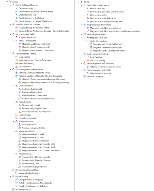
1 This physics interface is included with the core COMSOL package but has added functionality for this module.
2 This physics interface is a predefined multiphysics coupling that automatically adds all the physics interfaces and coupling features required.
3 Requires the addition of the Structural Mechanics Module or the MEMS Module.
4 Requires the addition of the Particle Tracing Module.
5 Requires the addition of the Structural Mechanics Module.
6 Requires the addition of the Multibody Dynamics Module.
7 Requires the addition of the Composite Materials Module.