The Wave Optics Module Physics Interfaces
The Wave Optics interfaces are based upon Maxwell’s equations together with material laws. In the module, these laws of physics are translated by the Wave Optics interfaces to sets of partial differential equations with corresponding initial and boundary conditions.
The Wave Optics interfaces define a number of features. Each feature represents a term or condition in the underlying Maxwell-based formulation and may be defined in a geometric entity of the model, such as a domain, boundary, edge (for 3D components), or point.
Figure 12 uses the Plasmonic Wire Grating application from the Wave Optics Module application library to show the Model Builder window and the Settings window for the selected Wave Equation, Electric 1 feature node. The Wave Equation, Electric 1 node adds terms representing the Helmholtz wave equation to the model equations for, in this case, all domains in the model. As this is an example of a periodic problem, the Wave Equation, Electric 1 node is a subnode to the Periodic Structure 1 node.
The Wave Equation, Electric 1 feature node may link to the Materials feature node to obtain physical properties such as relative permittivity and refractive index — in this case, the refractive index of a user-defined dielectric. The properties, defined by the Dielectric material, can be functions of the modeled physical quantities, such as temperature. Also the first material, Air, is in this case a user-defined material, whereas the third material, the gold wire (labeled Au (Rakic)), is taken from the Optical Material Library.
The simulation domain is delimited by boundary condition feature nodes. The default boundary condition feature for the physics interfaces in the Wave Optics Module is the Perfect Electric Conductor feature. For the example in Figure 12 the top Perfect Electric Conductor 1 feature node is overridden by the Periodic Structure 1 node. However, the Perfect Electric Conductor 1 subnode to the Periodic Structure 1 feature node is overridden by two Periodic Port feature nodes and a Floquet Periodic Condition feature node. The Periodic Port features are used for exciting and absorbing waves and the Floquet Periodic Condition relates fields on parallel opposing boundaries with Floquet periodicity conditions.
Figure 12: The Model Builder (left), and the Settings window for Wave Equation, Electric (right). The Equation section shows the model equations and the terms added by the Wave Equation, Electric 1 node to the model equations. The added terms are underlined with a dotted line. The text also explains the link between the Dielectric node and the values for the refractive index.
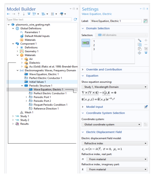
Figure 13 shows the Wave Optics interfaces, as displayed in the Model Wizard for this module.
Figure 13: The Wave Optics Module physics interfaces as displayed in the Model Wizard.
This module includes Wave Optics interfaces () for frequency-domain modeling and time-domain modeling, respectively. It also includes the Laser Heating interface, available under Heat Transfer. Also see Physics Interface Guide by Space Dimension and Study Type.
With the addition of the Semiconductor Module license, you also get the Semiconductor Optoelectronics, Beam Envelopes and The Semiconductor Optoelectronics, Frequency Domain interfaces that model the interaction of electromagnetic waves with semiconductors.
A brief overview of the Wave Optics interfaces follows.
Electromagnetic Waves, Frequency Domain
The Electromagnetic Waves, Frequency Domain interface () solves a frequency-domain wave equation for the electric field. The sources can be in the form of point dipoles, line currents, or incident fields on boundaries or domains. It is used primarily to model electromagnetic wave propagation in different media and structures. Variants of the formulation solves an eigenvalue problem to find the eigenfrequencies of a structure or, at a prescribed frequency, solves an eigenvalue problem to find the propagating modes in waveguides and transmission lines. Some typical applications that are simulated with the interface are waveguides, gratings, and scattering from small particles.
Electromagnetic Waves, Beam Envelopes
The Electromagnetic Waves, Beam Envelopes interface () solves one or two frequency-domain wave equations for the electric field envelope(s). The electric field is represented as the product of the solved for electric field envelope and a rapidly varying prescribed phase function. As the electric field envelopes has a slower spatial variation than the electric field, a coarse mesh can be used. Thus, the Electromagnetic Waves, Beam Envelopes interface is suitable for simulations of optically large structures (that is, structures that are much larger than the wavelength). The sources can be in the form of incident fields on boundaries, surface currents, or electric or magnetic fields on boundaries. The interface can be used for propagation problems at a fixed frequency and for finding eigenfrequencies in a resonant structure. Some typical applications that are simulated with the interface are waveguide structures, like directional couplers, nonlinear optical phenomena, and laser beam propagation.
Electromagnetic Waves, Boundary Elements
The Electromagnetic Waves, Boundary Elements interface () solves a frequency-domain wave equation for the electric field. The formulation is based on the boundary element method (BEM) and requires the availability of a Green’s function. Thus, the physics interface solves the vector Helmholtz equation for piecewise-constant material properties.
The interface is fully multiphysics enabled and can be coupled seamlessly with the physics interfaces that are based on the finite element method (FEM). This approach allows modeling in a FEM-BEM framework, using the strength of each formulation adequately. The BEM-based interface is especially well suited for radiation and scattering problems.
The advantage of the boundary element method is that only boundaries need to be meshed and the degrees of freedom (DOFs) solved for are restricted to the boundaries.
Electromagnetic Waves, Time Explicit
The Electromagnetic Waves, Time Explicit interface () solves a system of two first-order partial differential equations (Faraday’s law and Maxwell-Ampère’s law) for the electric and magnetic fields using the Time Explicit Discontinuous Galerkin method. The sources can be in the form of volumetric electric or magnetic currents or electric surface currents or fields on boundaries. It is used primarily to model electromagnetic wave propagation in linear media. Typical applications involve the transient propagation of electromagnetic pulses.
Electromagnetic Waves, Transient
The Electromagnetic Waves, Transient interface () solves a time-domain wave equation for the electric field. The sources can be in the form of point dipoles, line currents, or incident fields on boundaries or domains. It is used primarily to model electromagnetic wave propagation in different media and structures when a time-domain solution is required — for example, for nonsinusoidal waveforms or for nonlinear media. Typical applications involve the propagation of electromagnetic pulses and the generation of harmonics in nonlinear optical media.
Electromagnetic Waves, FEM-BEM
The Electromagnetic Waves, FEM-BEM multiphysics interface () allows to build hybrid FEM-BEM models, where the boundary element method (BEM) is used to compute the electric fields outside the finite element method (FEM) domains. This multiphysics interface adds an Electromagnetic Waves, Frequency Domain interface and an Electromagnetic Waves, Boundary Elements interface. The multiphysics coupling assures continuity of the tangential electric and magnetic fields across boundaries between the two interfaces.
Frequency-domain modeling is supported in 2D and 3D.
Laser Heating
The Laser Heating interface () is used to model electromagnetic heating for systems and devices where the electric field amplitude varies slowly on a wavelength scale. This multiphysics interface adds an Electromagnetic Waves, Beam Envelopes interface and a Heat Transfer in Solids interface. The multiphysics couplings add the electromagnetic losses from the electromagnetic waves as a heat source, and the electromagnetic material properties can depend on the temperature. The modeling approach is based on the assumption that the electromagnetic cycle time is short compared to the thermal time scale.
Combinations of frequency-domain modeling for the Electromagnetic Waves, Beam Envelopes interface and stationary modeling for the Heat Transfer in Solids interface, called frequency-stationary and, similarly, frequency-transient modeling, are supported in 2D and 3D.
Physics Interface Guide by Space Dimension and Study Type
The table below list the physics interfaces available specifically with this module in addition to the COMSOL Multiphysics basic license.
Heat Transfer
Electromagnetic Heating
Optics
Wave Optics
1 This physics interface is a predefined multiphysics coupling that automatically adds all the physics interfaces and coupling features required.