When adhesion is active, it is possible to break the bond between the source and destination boundaries by adding a Decohesion subnode to Contact. Decohesion modifies the stress vector f defined by Adhesion, but does not explicitly add any new contribution to the virtual work on the destination boundary. It thus requires an active Adhesion node.

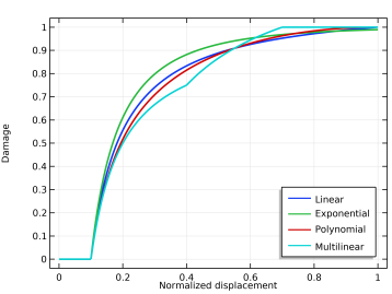
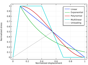
where d is the damage variable. During crack opening (or shearing), the damage variable grows, resulting in a softening behavior of the interface until it eventually breaks when d = 1, see Figure 3-43. If the interface is unloaded, the material follows the linear secant stiffness as defined by the current state of damage. No permanent deformations remain at complete unloading.

The Decohesion subnode implements the second term on the right-hand side of Equation 3-227, while the first term is implemented in Adhesion. Notice that in the normal direction, damage only applies to separation of the boundaries, hence the normal contact is unaffected by decohesion.

In the displacement-based damage models, the damage variable d is defined using a damage evolution function written in terms of a displacement quantity. Since, in general, the fracture is a combination of mode I and mode II fracture, the model introduces a mixed mode displacement um as the norm of the displacement jump vector.

To keep track of the current state of damage, the maximum value of um over the loading history is defined as

where is and internal degree of freedom that takes the value of um,max at the previous converged solution. The damage variable is then defined as a function of um,max of the form

where F–1 is called the damage evolution function and u0m defines the onset of damage. Conceptually, the damage evolution function is the inverse of the softening branch of the traction–separation law F. Four different definitions of the damage evolution function F−1 are available in the Traction–separation law list.

The damage evolution functions are summarized in Figure 3-42, and the resulting traction–separation laws in Figure 3-43.

The Linear option specifies a damage evolution function that gives a bilinear traction–separation law as seen in Figure 3-43. It is defined as

where u0m and ufm define the mixed mode initiation of damage and point of complete fracture, respectively. For the initiation of damage, a linear mixed mode criterion gives

where uI and uII are the mode I and mode II displacements, respectively. These are obtained from the displacement jump vector u. The constants u0t and u0s are calculated as

where σts is the tensile strength and σss is the shear strength of the adhesive layer. The normal stiffness kn and the equivalent tangential stiffness kt are obtained from the adhesive stiffness vector k. The mixed mode failure displacement ufm depends on the selected Mixed mode criterion.

The Power Law criterion is defined as

the Generalized Power Law criterion is defined as

and the Benzeggagh–Kenane criterion is defined as

where Gct, Gcs, and Gcm are the tensile, shear, and total energy release rates, respectively. The parameter α is called the mode mixity exponent. For the generalized power law criterion, the tensile and shear energy release rates have different mode mixity exponents, αt and αs respectively.

From these relations, the mixed mode failure displacement ufm is calculated. For the power law criterion it reads

where the mode mixity ratio reads β = uII/uI.

For the generalized power law criterion, the mixed mode failure displacement ufm is obtained after solving the nonlinear equation

and for the Benzeggagh–Kenane criterion, the corresponding expression for the mixed mode failure displacement ufm is

The Exponential option specifies a damage evolution function that gives a traction–separation law which is linear up to the interface strength, and thereafter softens with an exponential curve that asymptotically reaches zero as shown in Figure 3-43,

The mixed mode damage initiation displacement u0m is defined by Equation 3-228 and Equation 3-229.

The mixed mode failure displacement ufm reads for the power law

For the generalized power law criterion, the mixed mode failure displacement ufm is obtained after solving the nonlinear equation

and for the Benzeggagh–Kenane criterion, the mixed mode failure displacement ufm reads

The Polynomial option specifies a damage evolution function that gives a linear traction–separation law up to the interface strength, it thereafter softens with a cubic polynomial curve as shown in Figure 3-43,

The mixed mode damage initiation displacement u0m is defined by Equation 3-228 and Equation 3-229, and the mixed mode failure displacement ufm by Equation 3-230, Equation 3-231, or Equation 3-232.

The Multilinear option specifies a damage evolution function that gives a traction–separation law that is linear up to the interface strength. Thereafter a region of constant stress is introduced before the interface softens linearly as seen in Figure 3-43.

The mixed mode damage initiation displacement u0m is defined by Equation 3-228 and Equation 3-229.

The variable upm defines the end of the region of constant stress and introduces the shape factor λ. The shape factor defines the ratio between the constant stress part of Gct and the total “inelastic” part of Gct:

Note that the shape factor is similarly defined for shear and it is assumed to be equal for both components. Setting λ = 0 corresponds to the linear separation law.

Using the above expression, the stress plateau displacement, upi, for the respective component can be expressed as

and the failure displacement ufi as

where the index i indicates either tension or shear.

For the multilinear option, the mixed mode criterion is always linear (α = 1). Hence the mixed mode stress plateau displacement, upm, and the failure displacement, ufm, are given as

The energy-based damage models relate the growth of damage to the dissipated mechanical energy of the interface. The formulation is based on the work presented in Ref. 159 and Ref. 160. The derivation starts from the stored energy function

From the stored energy ψ(u, d), the stress vector f and damage energy release rate Ydm are obtained as

To keep track of the current state of damage, the maximum value of Yd over the loading history is defined as

where is an internal variable that takes the value of Ydm,max at the previous converged solution. The energy dissipated during the decohesion process is

where Gcm is the critical energy release rate in the sense of fracture mechanics. The overall behavior of the cohesive zone model is then summarized by

where Yd0m defines the damage threshold, and F(d) is a monotonically increasing function of the damage variable. From the above, an expression for the damage variable is obtained as

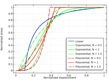
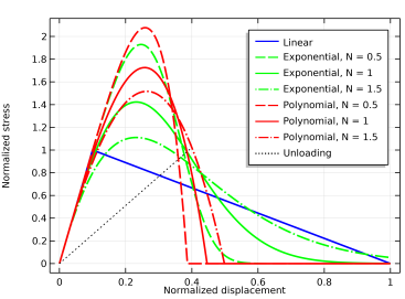
Different definitions for F−1 are available under the Traction–separation law list. These damage evolution functions are summarized in Figure 3-44, and the resulting traction–separation laws in Figure 3-45.

The Linear option specifies a damage evolution function that gives a bilinear traction–separation law as shown in Figure 3-45.

For the linear law, the equation constant Ydfm = Gcm.

The Exponential option specifies a more general damage evolution function of the form

where N is a smoothing parameter with a default value equal to 1. The effect of N on the traction–separation curve can be seen in Figure 3-45. For the exponential law, Ydfm is defined as

where Γ() is the gamma function.

A similar damage evolution function is obtained with the Polynomial option. It gives a generalized version of the traction–separation law proposed in Ref. 160,

The definition of the two variables, Yd0m and Gcm, requires the introduction of a few concepts related to the mixed mode loading. First, a mixed mode ratio is introduced

where uI and uII are the mode I and mode II displacements, respectively. These are obtained from the displacement jump vector u.

where G0t and G0s define the damage threshold in tension and shear, respectively.

where Gct and Gcs are the critical energy release rates for tension and shear, respectively. The variables α0 and αc are called the mode mixity exponents.

Such deficiencies may be alleviated by introducing some additional form of regularization. Under the Regularization list, it is possible to add the Delayed damage regularization. This option, available for time-dependent studies, adds a viscous delay to the damage growth. The formulation introduces a viscous damage variable dv. It redefines Equation 3-227 so that

where d is the damage variable obtained from any of the available CZM, and τ is the characteristic time that defines the delay of the decohesion. If the viscous damage is used to stabilize a rate-independent decohesion problem, the value of τ must be chosen with care. As a rule of thumb, τ should at least be one or two orders of magnitude smaller than the expected time step. Too large values of τ can introduce significant amounts of extra fracture energy to the model, and the actual energy dissipated due to damage can exceed the defined critical energy release rates by orders of magnitude.

The current value of the viscous damage variable, , is obtained after numerical integration of Equation 3-233 such that

where Δt is the current time step taken by the time-dependent solver. The value of the viscous damage at the previously converged step, , is stored as an internal variable.

where the required values at the previously converged step n are stored as internal variables.