Modeling with Layered Shells
A layered shell, also known as a composite laminate, is a thin-walled structure in 3D having many layers of different orthotropic (or optionally isotropic/anisotropic) material stacked on top of each other. A layered shell can be active either on free surfaces embedded in 3D or on the boundary of a solid object in 3D. In the latter case, it can be used to model a reinforcement on the surface of a solid object.
Figure 2-7: Geometry of a doubly curved laminated shell.
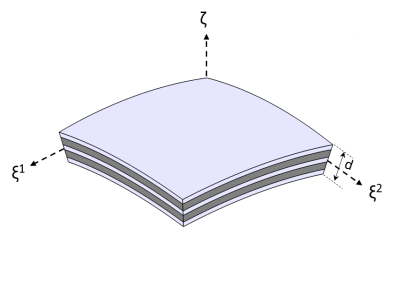
Figure 2-7 shows the uniform thickness doubly curved laminated shell having an orthogonal curvilinear coordinate system () and a total thickness (d).
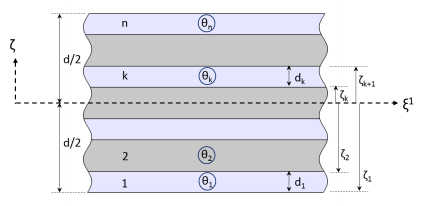
A typical stacking sequence of a composite laminate having n layers is shown in Figure 2-8. The thickness of each layer (dk), as well as the fiber direction in each layer (θk) with respect to first principal direction (ξ1) of the laminate are indicated. A counterclockwise rotation of the fiber direction with respect to the (ζ) direction is considered as positive.
Figure 2-8: A typical stacking sequence of a composite laminate showing thickness and fiber orientation in each layer.
For a general description of this section, see About Laminated Composite Shells in the documentation for the Composite Materials Module.
In COMSOL Multiphysics, layered shells can be analyzed either by the layerwise theory using the Layered Shell interface, or by the first order shear deformation theory (ESL-FSDT) theory using the Linear Elastic Material, Layered material model in the Shell interface. The layerwise theory of modeling a layered shell is discussed in the next section.
Physics Interface Selection
A Layered Shell physics interface is defined using a surface (2D) geometry and an extra dimension (1D) geometry in the through-thickness (or normal) direction. The surface geometry is a physical geometry and supposed to be created in the model whereas the extra dimension geometry is a virtual geometry created by Layered Material and similar nodes.
The geometric surface (or its lower dimension) selection, together with layer (or interface) selection creates the product geometry for the governing equations and boundary conditions of the Layered Shell interface.
The Layered Shell interface itself exists on a domain level which is a product geometry created using selected geometric surfaces and material layers. The physics features can exist on domain level or its lower dimensions. Based on whether a physics feature exists on a layer or an interface, the physics features can be divided into two categories:
Layer features may or may not allow a layer selection. When a layer selection is not allowed, the layer feature is applied to all layers.
Interface features, may allow only exterior interfaces, interior interfaces, or alternatively all interfaces of a laminate.
For a general description of layer selections, see Layer and Interface Selections in the documentation for the Composite Materials Module.
For a general description of layered materials, see Layered Materials in the documentation for the Composite Materials Module.
Layer Materials, Thicknesses, and Orientations
A layered shell can have many layers with following different properties in each layer:
For a general description of layered materials, see Layered Materials in the documentation for the Composite Materials Module.
Offset and Local Coordinate System
The position of the reference surface with respect to midplane of the laminate and the local coordinate system in which material properties and results are interpreted can be defined in Layered Material and similar nodes.
For a general description of layered materials, see Layered Materials in the documentation for the Composite Materials Module.
Transform and Scale
The transform functionality can be optionally used to simplify the definition of stacking sequence. Various transform options available are symmetric, antisymmetric, and repeated.
The scale functionality can be optionally used to model a variable thickness layer. The scale defined for each layer, which could be a function of reference geometry, is multiplied to the constant layer thickness essentially making it a variable thickness layer.
The transform and scale options can be defined in Layered Material and similar nodes.
For a general description of layered materials, see Layered Materials in the documentation for the Composite Materials Module.
Using the Extra Dimension Coordinates
Sometimes, you want to write expressions that are functions of the coordinates in the thickness direction of the layered shell. If you write expressions based on the usual coordinates, like X, Y, and Z, such an expression will be evaluated on the reference surface (the meshed boundaries). In addition to this, you can access locations in the through-thickness direction by making explicit or implicit use of the coordinates in the extra dimension.
The extra dimension coordinate has a name like x_llmat1_xdim. The middle part of the coordinate name is derived from the tag of the layered material definition where it is created; in this example a Layered Material Link.
You can also access the extra dimension coordinate as wrapped into a physics interface variable, like lshell.xd (varies from 0 to the total laminate thickness d) and lshell.xd_rel (varies from 0 to 1).
Finally, the coordinates in 3D space are available using the physics scoped variables lshell.X, lshell.Y, and lshell.Z. These coordinates vary also in the thickness direction of the layered shell.
You can also write expressions that explicitly contain the number of the layer, available in the variable lshell.num. The number of the bottommost layer is ‘1’.
Results Evaluation in Layered Shells
For visualization and results evaluation, predefined variables include all nonzero stress and strain tensor components, principal stresses and principal strains, in-plane and out-of-plane forces, moments, and von Mises and Tresca equivalent stresses.
Stresses and strains are available in the global coordinate system, laminate coordinate system, as well as in the layer local coordinate system.
Layered Material Slice Plot
It is possible to evaluate the stress and strain tensor components and equivalent stresses in each layer of a laminate using Layered Material Slice plot.
The through-thickness location can be set to evaluate a quantity in the middle of a layer, at an interface between two layers, top or bottom of a laminate, and so on. The top, bottom, and the middle of a laminate can be defined as:
Bottom of a laminate: 1 (relative) and 0 (physical)
Middle of a laminate: 0 (relative) and d/2 (physical)
Top of a laminate: +1 (relative) and d (physical)
The default value for the through-thickness location is given in the Default through-thickness result location section of the Layered Shell interface.
Through Thickness Plot
The through-thickness variation of a quantity at one or more locations on the reference surface can be plotted using a Through Thickness plot. In this plot, the reference surface locations can be specified through following ways:
Layered Material Dataset
The Layered Material dataset allows the display of results in 3D solid even though the equations are solved on a 2D surface.
Using this dataset, results can either be visualized on a 3D object or on slices created in the through-thickness direction of a 3D object. The following options are available in the dataset to create slices in the through-thickness direction:
Sometimes, when a laminate is very thin, it becomes difficult to distinguish between a surface or a solid object. In such cases it is possible to scale the through-thickness direction in the dataset for better visualization.
In order to use the section stiffness approach, you must obtain all terms in the stiffness matrix. In the case of dynamic analysis, also inertial matrices are needed. For some common cases, like perforation and corrugation, expressions for these quantities may be found in the literature. In general, however, you have to set up a finite element model of a representative part of the structure, and compute the homogenized data based on the results from various load cases.
Given only the homogenized stiffness and computed deformations, there is not enough information to compute stresses. The stress state will depend on the local geometry. In the Section Stiffness node, you have a possibility to define expressions for the relation between section forces and stresses. Such expressions must then be based on your knowledge of the peak stresses in the original, not homogenized structure. As an example, for a perforated structure, the stress concentrations around the holes should be taken into account.