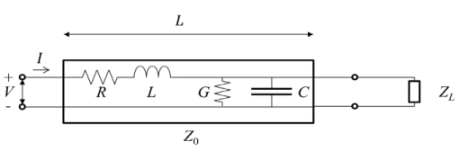
Figure 4-9 is an illustration of a transmission line of length
L. The distributed resistance
R, inductance
L, conductance
G, and capacitance
C, characterize the properties of the transmission line.
The distribution of the electric potential V and the current
I describes the propagation of the signal wave along the line. The following equations relate the current and the electric potential
Equation 4-1 and
Equation 4-2 can be combined to the second-order partial differential equation
Here γ,
α, and
β are called the complex propagation constant, the attenuation constant, and the (real) propagation constant, respectively.
The solution to Equation 4-3 represents a forward- and a backward-propagating wave
By inserting Equation 4-4 in
Equation 4-1 the current distribution is obtained.