Introduction
The Pipe Flow Module is an optional add-on package for COMSOL Multiphysics designed to model and simulate fluid flow, heat, and mass transfer in pipes and channels. Compressible hydraulic transients and acoustic waves can also be modeled using the Water Hammer interface and Pipe Acoustics interface, respectively. To analyze the stresses and deformation in the pipes, the Pipe Mechanics interface is available. The Pipe Flow Module can address problems involving flow velocity, pressure, temperature, stresses, deformation, and sound waves in pipes and channels.
Modeling pipes as curves in 2D or 3D gives a great advantage in computational efficiency over meshing and computing 3D pipes with finite diameter.
Figure 1: The Pipe Flow interface reduces the 3D flow problem to a 2D or 3D curve.
Pipe systems for which the ratio length/diameter is large enough that the flow inside of each pipe segment can be considered fully developed are suitable for the Pipe Flow Module.
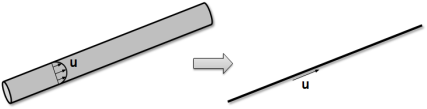
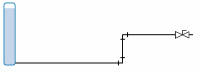
The physics interfaces in the module define the conservation of momentum, energy, and mass of a fluid inside a pipe or channel. The flow rate, pressure, temperature, and concentration fields are modeled as cross-section averaged quantities, so that they only vary along the length of the pipes. The pressure losses along the length of a pipe or in a pipe component are described using friction factors. A broad range of built-in expressions for Darcy and Fanning friction factors cover the entire flow regime from laminar to turbulent flow, Newtonian and non-Newtonian fluids, different cross-sectional geometries, and a wide range of relative surface roughness values. In addition to the continuous frictional pressure drop along pipe stretches, pressure drops due to irreversible losses in components such as bends, contractions, expansions, T-junctions, Y-junctions, and valves are computed through an extensive library of industry standard loss coefficients. Pumps are also available as flow inducing devices.
The features in this module are intended for modeling and simulating incompressible and weakly compressible fluid flow in pipes and channel systems, as well as compressible hydraulic transients and acoustic waves. Typical simulations yield the velocity, pressure variation, and temperature in systems of pipes and channels. Hydraulic transients are also possible to model. These can be the result of a valve that is closed rapidly in a pipe network, which is referred to as a water hammer.
The Pipe Mechanics interface is intended for modeling slender pipes with arbitrary cross sections. Among the computed results are displacements, rotations, stresses, strains, and section forces.
The Applications
The module can be used to design and optimize complex cooling systems in turbines, analyze ventilation systems in buildings, pipe systems in the chemical process industry, and pipelines in the oil and gas industry, just to mention a few applications.
Figure 2: A Probe Tube Microphone modeled using the “Pipe Acoustics, Transient” interface in the Pipe Flow Module.
Any devices in which you find flow, waves, or mass or heat-transfer phenomena in narrow pipes or ducts are candidates for simulation with the Pipe Flow Module. Classical pressure-drop and mass flow calculations through piping with bends, valves, tanks, and so forth are well suited for the Pipe Flow Module.
Figure 3: Tutorial model describing the discharging of a water tank through a simple pipe system with bends and valves.
For heat transfer studies, the Pipe Flow Module includes several automatic couplings to the surrounding heat sinks or sources; both shortcut methods with semi-empirical correlations for forced and convection, and also direct coupling to a 3D solid, in which the pipe is embedded.
Figure 4: Methods for heat transfer to the surroundings, from left to right: forced convection, natural convection, solid conduction.
An example of an application which demonstrates the capabilities of pipe-solid coupling is the Mold Cooling model in the Pipe Flow application library. When manufacturing devices in polymeric materials, the structural integrity of the end product is very sensitive to the cooling history in the mold.
Figure 5: The heat transfer to the cooling channels embedded in a cooling mold is simulated to understand the controlled cooling of a polyurethane steering wheel. The Nonisothermal Pipe Flow interface is used in the model.
With the capabilities of modeling the transfer of chemical compounds diluted in fluids flowing through thin pipes, the pipe flow module allows for complex chemical reaction modeling. This can include mass transfer, chemical kinetics, heat transfer, and pressure drop calculations in the same model.
Figure 6: Temperature distribution in an autothermal chemical reactor. The model includes mass transport, chemical kinetics, heat transfer, and pressure drop and flow calculations.
Thanks to COMSOL Multiphysics’ strong capabilities in handling nonlinear materials, such as non-Newtonian fluids and materials with highly temperature-dependent physical properties, oil and gas applications can be readily modeled. One example is crude oil pipelines, where the viscous heating effects combined with the temperature dependent viscosity have great impact on the possibilities to convey oil through pumping.
Figure 7: The Pipeline Insulation model in the application library simulates the effect of viscous heating on the cooling and transport properties of oil in a pipeline.
The Pipe Connection multiphysics coupling feature can connect a pipe segment to a 3D flow domain seamlessly and easily.