|
|
|


|
1
|
|
2
|
|
3
|
Click Add.
|
|
4
|
Click
|
|
5
|
|
6
|
Click
|
|
1
|
|
2
|
|
3
|
|
1
|
|
2
|
|
1
|
|
2
|
|
3
|
|
4
|
Locate the Units section. In the table, enter the following settings:
|
|
5
|
|
1
|
|
2
|
|
3
|
|
4
|
Locate the Units section. In the table, enter the following settings:
|
|
5
|
|
1
|
|
2
|
|
3
|
|
4
|
Locate the Units section. In the table, enter the following settings:
|
|
5
|
|
1
|
|
2
|
|
3
|
|
4
|
|
5
|
|
6
|
|
7
|
Click
|
|
8
|
|
1
|
|
2
|
Go to the Add Material window.
|
|
3
|
|
4
|
Click Add to Component in the window toolbar.
|
|
5
|
|
1
|
|
2
|
|
1
|
Right-click Component 1 (comp1) > Electromagnetic Waves, Transient (ewt) and choose Perfect Magnetic Conductor.
|
|
1
|
|
3
|
In the Settings window for Scattering Boundary Condition, locate the Scattering Boundary Condition section.
|
|
4
|
|
5
|
|
1
|
|
1
|
|
2
|
|
3
|
|
4
|
|
1
|
|
3
|
|
4
|
|
5
|
In the Relative placement of vertices along edge text field, type sin(range(0,0.025*pi,0.5*pi)). This creates a denser mesh closer to the upper boundary.
|
|
1
|
|
2
|
|
3
|
Click the Custom button.
|
|
4
|
|
5
|
Click
|
|
6
|
|
1
|
|
2
|
|
3
|
|
1
|
In the Model Builder window, expand the Domain Point Probe 1 node, then click Point Probe Expression 1 (ppb1).
|
|
2
|
|
3
|
Click Replace Expression in the upper-right corner of the Expression section. From the menu, choose Component 1 (comp1) > Electromagnetic Waves, Transient > Electric > Electric field - V/m > ewt.Ez - Electric field, z-component.
|
|
1
|
|
2
|
|
3
|
|
4
|
|
1
|
|
2
|
|
3
|
|
4
|
|
5
|
|
6
|
In the Model Builder window, expand the Study 1 > Solver Configurations > Solution 1 (sol1) > Time-Dependent Solver 1 node, then click Fully Coupled 1.
|
|
7
|
|
8
|
Select the Use linear heuristics for adaptive tolerance checkbox.
|
|
9
|
|
1
|
|
2
|
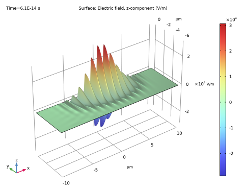
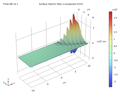
In the Settings window for Surface, click Replace Expression in the upper-right corner of the Expression section. From the menu, choose ewt.Ez - Electric field, z-component - V/m.
|
|
1
|
|
2
|
|
4
|
|
1
|
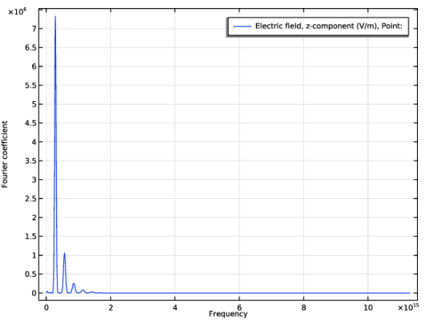
In the Model Builder window, expand the Results > Probe Plot Group 1 node, then click Probe Table Graph 1.
|
|
2
|
|
3
|
|
4
|
|
5
|
Select the Frequency range checkbox.
|
|
6
|