|
|
|

|
1
|
|
2
|
In the Select Physics tree, select Optics > Wave Optics > Electromagnetic Waves, Frequency Domain (ewfd).
|
|
3
|
Click Add.
|
|
4
|
Click
|
|
5
|
In the Select Study tree, select Preset Studies for Selected Physics Interfaces > Wavelength Domain.
|
|
6
|
Click
|
|
1
|
|
2
|
Browse to the model’s Application Libraries folder and double-click the file photonic_crystal_demultiplexer_optimization_geom_sequence.mph.
|
|
3
|
|
4
|
|
5
|
|
6
|
|
1
|
In the Model Builder window, under Component 1 (comp1) right-click Materials and choose Blank Material.
|
|
2
|
|
3
|
Locate the Material Contents section. In the table, enter the following settings:
|
|
1
|
|
2
|
Go to the Add Material window.
|
|
3
|
In the tree, select Optical > Inorganic Materials > As - Arsenides > Experimental data > GaAs (Gallium arsenide) (Papatryfonos et al. 2021: n,k 0.260-1.88 um).
|
|
4
|
Click Add to Component in the window toolbar.
|
|
5
|
|
1
|
|
2
|
|
1
|
In the Model Builder window, under Component 1 (comp1) click Electromagnetic Waves, Frequency Domain (ewfd).
|
|
2
|
|
3
|
|
1
|
|
2
|
|
3
|
|
1
|
|
2
|
|
3
|
|
4
|
Locate the Scattering Boundary Condition section. From the Incident field list, choose Wave given by E field.
|
|
5
|
|
1
|
|
2
|
|
3
|
|
4
|
|
5
|
|
6
|
Click Replace Expression in the upper-right corner of the Expression section. From the menu, choose Component 1 (comp1) > Electromagnetic Waves, Frequency Domain > Energy and power > ewfd.nPoav - Power outflow, time average - W/m².
|
|
1
|
|
2
|
|
3
|
|
4
|
|
1
|
|
2
|
|
3
|
Locate the Parameters section. In the table, enter the following settings:
|
|
1
|
|
2
|
|
3
|
From the list, choose User-controlled mesh.
|
|
1
|
|
2
|
|
3
|
|
4
|
|
5
|
|
1
|
|
2
|
|
3
|
|
4
|
|
5
|
|
6
|
Clear the Maximum element growth rate checkbox.
|
|
7
|
Clear the Curvature factor checkbox.
|
|
8
|
Clear the Resolution of narrow regions checkbox.
|
|
9
|
Click
|
|
1
|
|
2
|
|
3
|
|
4
|
|
5
|
|
6
|
|
7
|
|
8
|
|
1
|
|
2
|
|
3
|
Click
|
|
4
|
Click
|
|
5
|
|
6
|
Click OK.
|
|
1
|
|
2
|
|
3
|
|
4
|
Locate the Translation section. In the table, enter the following settings:
|
|
5
|
|
1
|
In the Model Builder window, under Component 1 (comp1) right-click Definitions and choose Variables.
|
|
2
|
|
3
|
Locate the Variables section. In the table, enter the following settings:
|
|
1
|
|
2
|
Go to the Add Study window.
|
|
3
|
Find the Studies subsection. In the Select Study tree, select Preset Studies for Selected Physics Interfaces > Wavelength Domain.
|
|
4
|
Click Add Study in the window toolbar.
|
|
5
|
|
6
|
Click Add Study in the window toolbar.
|
|
7
|
|
1
|
|
2
|
In the Solve for column of the table, under Component 1 (comp1), select the checkbox for Electromagnetic Waves, Frequency Domain (ewfd).
|
|
3
|
In the Solve for column of the table, under Component 1 (comp1), clear the checkbox for Deformed Geometry.
|
|
1
|
|
2
|
|
3
|
In the Wavelengths text field, type range(lambda3-dWave3/2,dWave/(dWaveN3-1),lambda3+dWave3/2) range(lambda1-dWave/2,dWave/(dWaveN-1),lambda1+dWave/2) range(lambda4-dWave4/2,dWave4/(dWaveN4-1),lambda4+dWave4/2) range(lambda2-dWave/2,dWave/(dWaveN-1),lambda2+dWave/2) range(lambda5-dWave5/2,dWave5/(dWaveN5-1),lambda5+dWave5/2) range(lambda6-dWave6/2,dWave6/(dWaveN6-1),lambda6+dWave6/2).
|
|
4
|
|
1
|
|
2
|
|
3
|
|
4
|
Click Add Expression in the upper-right corner of the Objective Function section. From the menu, choose Component 1 (comp1) > Definitions > Variables > comp1.obj - Objective function - 1.
|
|
5
|
|
6
|
|
7
|
|
8
|
|
9
|
|
10
|
|
11
|
|
12
|
Select the Plot checkbox.
|
|
13
|
|
1
|
In the Model Builder window, expand the Shape Optimization > Solver Configurations > Solution 2 (sol2) node, then click Optimization Solver 1.
|
|
2
|
|
3
|
|
4
|
In the Model Builder window, expand the Shape Optimization > Solver Configurations > Solution 2 (sol2) > Optimization Solver 1 > Stationary Solver 1 node.
|
|
5
|
|
6
|
|
7
|
|
8
|
|
9
|
|
10
|
Locate the General section. In the Variables list, select Electric Field (Spatial and Material Frames) (comp1.E).
|
|
11
|
|
12
|
In the Model Builder window, under Shape Optimization > Solver Configurations > Solution 2 (sol2) > Optimization Solver 1 > Stationary Solver 1 > Segregated 1 click Segregated Step 1.
|
|
13
|
|
14
|
|
15
|
In the Add dialog, in the Variables list, choose Electric Field (Spatial and Material Frames) (comp1.E) and Translation (Geometry Frame) (comp1.tsf1.move).
|
|
16
|
Click OK.
|
|
17
|
|
1
|
|
2
|
Right-click Results > Datasets > Shape Optimization/Solution 2 (sol2) and choose Remesh Deformed Configuration.
|
|
1
|
|
2
|
In the Solve for column of the table, under Component 1 (comp1), clear the checkbox for Deformed Geometry.
|
|
3
|
Click to expand the Values of Dependent Variables section. Find the Initial values of variables solved for subsection. From the Settings list, choose User controlled.
|
|
4
|
|
5
|
|
6
|
Find the Values of variables not solved for subsection. From the Settings list, choose User controlled.
|
|
7
|
|
8
|
|
9
|
Click to expand the Store in Output section. In the table, enter the following settings:
|
|
11
|
|
12
|
|
13
|
Click OK.
|
|
14
|
|
17
|
|
18
|
|
19
|
Click OK.
|
|
20
|
|
22
|
|
23
|
|
24
|
|
25
|
|
1
|
|
2
|
|
1
|
|
2
|
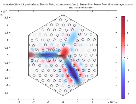
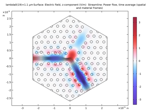
In the Settings window for Surface, click Replace Expression in the upper-right corner of the Expression section. From the menu, choose Component 1 (comp1) > Electromagnetic Waves, Frequency Domain > Electric > Electric field - V/m > ewfd.Ez - Electric field, z-component.
|
|
3
|
|
1
|
|
2
|
In the Settings window for Streamline, click Replace Expression in the upper-right corner of the Expression section. From the menu, choose Component 1 (comp1) > Electromagnetic Waves, Frequency Domain > Energy and power > ewfd.Poavx,ewfd.Poavy - Power flow, time average (spatial and material frames).
|
|
3
|
|
4
|
Locate the Coloring and Style section. Find the Line style subsection. From the Type list, choose Tube.
|
|
5
|
Select the Radius scale factor checkbox.
|
|
6
|
|
1
|
|
2
|
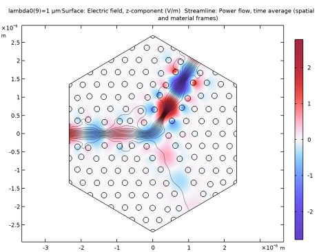
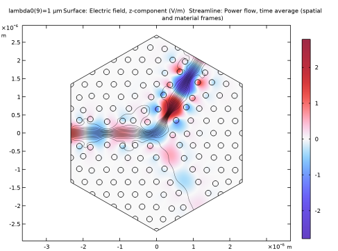
In the Settings window for Surface, click Replace Expression in the upper-right corner of the Expression section. From the menu, choose Component 1 (comp1) > Electromagnetic Waves, Frequency Domain > Electric > Electric field (spatial and material frames) - V/m > ewfd.Ez - Electric field, z-component.
|
|
3
|
|
4
|
|
1
|
|
2
|
|
3
|
|
4
|
|
5
|
|
6
|
|
7
|
|
1
|
|
2
|
|
3
|
|
4
|
|
5
|
Locate the Plot Settings section.
|
|
6
|
|
7
|
|
8
|
|
9
|
|
1
|
|
2
|
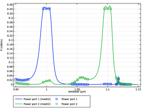
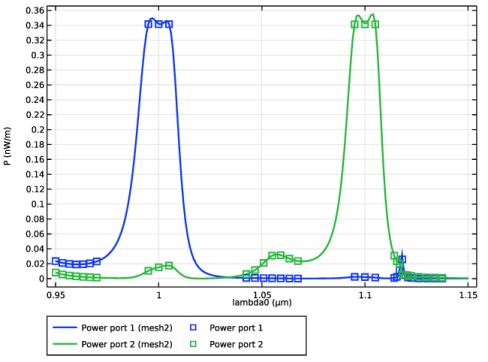
In the Settings window for Global, click Add Expression in the upper-right corner of the y-Axis Data section. From the menu, choose Component 1 (comp1) > Definitions > obj1 - Power Port 1 - W/m.
|
|
3
|
Click Add Expression in the upper-right corner of the y-Axis Data section. From the menu, choose Component 1 (comp1) > Definitions > obj2 - Power Port 2 - W/m.
|
|
4
|
Locate the y-Axis Data section. In the table, enter the following settings:
|
|
5
|
|
6
|
|
1
|
|
2
|
|
3
|
|
4
|
Locate the Coloring and Style section. Find the Line style subsection. From the Line list, choose None.
|
|
5
|
|
6
|
|
7
|
Locate the y-Axis Data section. In the table, enter the following settings:
|
|
8
|
|
9
|
|
1
|
|
2
|
|
3
|
|
1
|
|
2
|
|
3
|
|
4
|
|
5
|
Select the Radius scale factor checkbox.
|
|
1
|
|
2
|
|
3
|
|
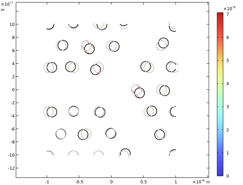
1
|
|
2
|
In the Settings window for Deformation, click Replace Expression in the upper-right corner of the Expression section. From the menu, choose Component 1 (comp1) > Definitions > Transformation 1 > tsf1.dXg,tsf1.dYg - Boundary displacement (geometry frame).
|
|
3
|
|
4
|
|
5
|
Locate the Scale section.
|
|
6
|
|
1
|
In the Model Builder window, expand the Results > Thumbnail > Translation (Transformation 1) node, then click Color Expression 1.
|
|
2
|
|
3
|
|
4
|
|
1
|
|
2
|
|
3
|
|
4
|
|
1
|
|
2
|
|
3
|
|
4
|
|
5
|
|
1
|
|
2
|
|
1
|
|
2
|
|
4
|
Locate the Selections of Resulting Entities section. Select the Resulting objects selection checkbox.
|
|
1
|
|
2
|
|
3
|
|
4
|
|
5
|
|
6
|
Locate the Selections of Resulting Entities section. Select the Resulting objects selection checkbox.
|
|
1
|
|
2
|
|
3
|
|
4
|
Select the Keep input objects checkbox.
|
|
5
|
|
6
|
|
1
|
|
2
|
|
3
|
|
4
|
|
5
|
|
6
|
|
7
|
|
1
|
|
2
|
|
3
|
|
1
|
|
2
|
|
3
|
|
4
|
|
5
|
|
6
|
|
1
|
|
2
|
|
3
|
|
4
|
|
1
|
In the Model Builder window, under Component 1 (comp1) > Geometry 1 right-click Circles to Delete, Row 1 (boxsel2) and choose Duplicate.
|
|
2
|
|
1
|
In the Model Builder window, under Component 1 (comp1) > Geometry 1 right-click Circles to Delete, Row 2 (boxsel3) and choose Duplicate.
|
|
2
|
|
1
|
|
2
|
|
3
|
|
4
|
In the Add dialog, in the Selections to add list, choose Circles to Delete, Row 1, Circles to Delete, Row 2, and Circles to Delete, Row 3.
|
|
5
|
Click OK.
|
|
1
|
|
2
|
|
3
|
|
4
|
|
1
|
|
2
|
|
3
|
|
1
|
|
2
|
|
3
|
|
4
|
|
5
|
Click OK.
|
|
6
|
|
7
|
|
8
|
|
9
|
Click OK.
|
|
1
|
|
2
|
|
3
|
|
4
|
|
1
|
|
2
|
|
3
|
|
4
|
|
5
|
|
6
|
|
7
|
|
8
|
|
9
|
Locate the Selections of Resulting Entities section. Select the Resulting objects selection checkbox.
|
|
1
|
|
2
|
|
3
|
|
4
|
|
5
|
|
6
|
|
1
|
|
2
|
|
3
|
Locate the Starting Point section. In the y text field, type (-W/2*2/sqrt(3)-sin(1/6*pi)*W/2*2/sqrt(3))/2-dPeriod/2*sin(-pi*5/6).
|
|
4
|
Locate the Endpoint section. In the y text field, type (-W/2*2/sqrt(3)-sin(1/6*pi)*W/2*2/sqrt(3))/2+dPeriod/2*sin(-pi*5/6).
|
|
1
|
|
2
|
|
3
|
|
4
|
|
5
|
Click OK.
|
|
1
|
|
2
|
|
3
|
|
4
|
|
5
|
Click OK.
|
|
1
|
|
2
|
|
3
|
|
4
|
Click
|
|
5
|
|
6
|
Click OK.
|
|
7
|
|
8
|
|
1
|
|
2
|
|
3
|
|
4
|
|
5
|
Click OK.
|
|
1
|
|
2
|
|
1
|
|
2
|
|
3
|