PDF

Acousto-Optic Modulator
Introduction
The refractive index of an optical material is altered by mechanical stress, as is demonstrated in the application library example Stress–Optical Effects in a Photonic Waveguide. In that example, the mechanical stress is applied statically. However, the refractive index is also altered by rapidly varying mechanical stress, as applied by a sound wave propagating in the optical material. The interaction between light and sound is called acousto-optics.
The acousto-optic effect can be used for modulation of laser beam power or frequency or for deflection of a laser beam. An acousto-optic modulator (AOM) is a device that modulates the power of the laser beam that passes through the device.
The AOM consists of a transparent crystal (or piece of glass), through which the light propagates. A piezoelectric transducer, attached to the crystal, is used to excite a sound wave with a frequency of the order of 100 MHz. Light can then experience Bragg diffraction by the traveling periodic refractive index grating generated by the sound wave. Therefore, AOMs are sometimes called Bragg cells.
Some of the applications for AOMs include:
Since the diffraction angle depends on the acoustic frequency, one can scan the output beam direction by changing the modulation frequency. This is useful for deflector (scanning) applications.
This example demonstrates the basic physics principles for an AOM, with just a single refractive index period. Manufactured components are much larger and can be modeled with the same principle as the Ray Optics Module Application Library example Diffraction Grating.
Model Definition
This model uses the Solid Mechanics interface with a Frequency Domain study, to model the sound wave. Thus, any of the following licenses are needed to run this model:
First, the acoustic (sound) problem is solved. In a subsequent step, the optical problem is solved, using the Electromagnetic Waves, Frequency Domain interface. To model the periodic problem, the Periodic Structure node is added. It simplifies the process of setting up the ports for exciting and absorbing the light wave and for defining the periodic boundary conditions.
As discussed in more detail in the application library example Stress–Optical Effects in a Photonic Waveguide, the refractive index relates to the stress by
,
where nx, ny, and nz are the diagonal elements of the refractive index tensor and, similarly, Sx, Sy, and Sz are the diagonal elements of the stress tensor.
Results and Discussion
Figure 1 shows the mechanical stress field, that induces the modulation of the refractive index.
Figure 1: The mechanical stress field.
Figure 2 shows that the mechanical displacement in the sound wave is in the nm range.
Figure 2: The mechanical displacement field in the x direction.
Figure 3 shows that due to the induced refractive index grating, higher diffraction orders are excited.
Figure 3: The z-component of the electric field of the optical wave.
Figure 4 visualizes the different mode fields involved on the transmission side, by spatially separating them for clarity.
Figure 4: A visualization of the mode fields on the transmission side. The central wave is the normally propagating m = 0 mode, whereas the obliquely propagating waves represent the m = -1 (left) and m = 1 (right) modes. The mode fields are multiplied by the respective S-parameters, to make the waves have the field strength as in the full solution in Figure 3.
Application Library path: Wave_Optics_Module/Modulators_and_Switches/acousto_optic_modulator
Modeling Instructions
From the File menu, choose New.
New
In the New window, click  Model Wizard.
Model Wizard
1
In the Model Wizard window, click  2D.
2
In the Select Physics tree, select Structural Mechanics > Solid Mechanics (solid).
3
Click Add.
4
In the Select Physics tree, select Optics > Wave Optics > Electromagnetic Waves, Frequency Domain (ewfd).
5
Click Add.
6
Click  Study.
7
In the Select Study tree, select General Studies > Frequency Domain.
8
Global Definitions
First load some parameters that define geometry dimensions, material properties, and properties used by the physics interfaces.
Parameters 1
1
In the Model Builder window, under Global Definitions click Parameters 1.
2
In the Settings window for Parameters, locate the Parameters section.
3
Click  Load from File.
4
Notice that the wavelengths and frequencies are different for the acoustic and optical waves.
Geometry 1
Rectangle 1 (r1)
1
In the Geometry toolbar, click  Rectangle.
2
In the Settings window for Rectangle, locate the Size and Shape section.
3
In the Width text field, type a.
4
In the Height text field, type b.
5
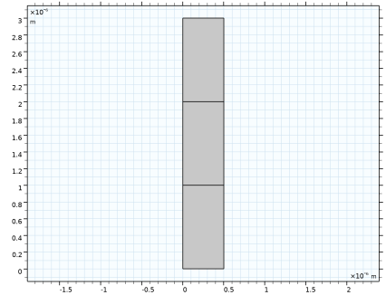
Click to expand the Layers section. In the table, enter the following settings:
6
Select the Layers on top checkbox.
7
Click  Build All Objects.
This creates a rectangular geometry, consisting of three layers. Air will be assigned to the top domain. The two domains below, will use SiO2. However, the acoustic wave will only propagate through (and modulate) the middle domain.
Materials
Air
1
In the Model Builder window, under Component 1 (comp1) right-click Materials and choose Blank Material.
2
In the Settings window for Material, type Air in the Label text field.
3
Locate the Material Contents section. In the table, enter the following settings:
This is the only material property that needs to be added to this material, as this material will not be used by the Solid Mechanics interface.
SiO2, Acousto-Optics
Now, add the acousto-optic material, where the mechanical stress will induce a modulation of the refractive index.
1
Right-click Materials and choose Blank Material.
2
In the Settings window for Material, type SiO2, Acousto-Optics in the Label text field.
3
4
Locate the Material Contents section. In the table, enter the following settings:
5
6
Right-click the Refractive index, real part row and choose Edit.
7
In the Refractive index, real part dialog, choose Diagonal from the list.
8
9
SiO2, Plain
Finally, add the plain SiO2 material, where there is no acousto-optic interaction.
1
Right-click SiO2, Acousto-Optics and choose Duplicate.
2
In the Settings window for Material, type SiO2, Plain in the Label text field.
3
4
Locate the Material Contents section. Click to select row number 4 in the table.
5
Right-click the Refractive index, real part row and choose Edit.
6
In the Refractive index, real part dialog, choose Isotropic from the list.
7
8
Solid Mechanics (solid)
1
In the Model Builder window, under Component 1 (comp1) click Solid Mechanics (solid).
2
Prescribed Displacement 1
Add the boundary that will vibrate and generate the acoustic wave.
1
In the Physics toolbar, click  Boundaries and choose Prescribed Displacement.
2
3
In the Settings window for Prescribed Displacement, locate the Prescribed Displacement section.
4
From the Displacement in x direction list, choose Prescribed.
5
In the u0x text field, type 0.01[nm].
6
From the Displacement in y direction list, choose Prescribed.
Fixed Constraint 1
1
In the Physics toolbar, click  Boundaries and choose Fixed Constraint.
2
Symmetry 1
1
In the Physics toolbar, click  Boundaries and choose Symmetry.
2
Electromagnetic Waves, Frequency Domain (ewfd)
1
In the Model Builder window, under Component 1 (comp1) click Electromagnetic Waves, Frequency Domain (ewfd).
2
In the Settings window for Electromagnetic Waves, Frequency Domain, locate the Components section.
3
From the Electric field components solved for list, choose Out-of-plane vector, as the optical wave will be polarized in the z-direction.
Periodic Structure 1
1
In the Physics toolbar, click  Domains and choose Periodic Structure.
2
In the Settings window for Periodic Structure, locate the Port Mode Settings section.
3
In the α text field, type alpha.
4
Locate the Port Handling section. Click Add Diffraction Orders, to generate all the necessary diffraction orders to absorb all radiation that reaches the port boundaries.
Mesh 1
Create a mesh that makes sure that the mesh is exactly the same on the parallel opposing edges, where the Floquet Periodic Condition ìs applied.
Identical Mesh 1
1
In the Mesh toolbar, click  More Attributes and choose Identical Mesh.
2
3
In the Settings window for Identical Mesh, locate the Second Entity Group section.
4
Click to select the  Activate Selection toggle button.
5
Free Triangular 1
In the Mesh toolbar, click  Free Triangular.
Size
1
In the Model Builder window, click Size.
2
In the Settings window for Size, click to expand the Element Size Parameters section.
3
In the Maximum element size text field, type lam0/N/10.
4
Click  Build All.
Study 1: Stress and Strain
1
In the Model Builder window, click Study 1.
2
In the Settings window for Study, type Study 1: Stress and Strain in the Label text field.
Step 1: Frequency Domain
1
In the Model Builder window, under Study 1: Stress and Strain click Step 1: Frequency Domain.
2
In the Settings window for Frequency Domain, locate the Physics and Variables Selection section.
3
In the Solve for column of the table, under Component 1 (comp1), clear the checkbox for Electromagnetic Waves, Frequency Domain (ewfd), to only solve for the Solid Mechanics interface in this study step.
4
Locate the Study Settings section. From the Frequency unit list, choose GHz.
5
In the Frequencies text field, type freq_disp.
6
In the Study toolbar, click  Compute.
Results
Height Expression 1
1
In the Model Builder window, expand the Stress (solid) node.
2
Right-click Surface 1 and choose Height Expression.
3
In the Settings window for Height Expression, locate the Axis section.
4
Select the Scale factor checkbox. In the associated text field, type 1.5E-17.
Deformation
1
In the Model Builder window, right-click Deformation and choose Disable.
2
In the Stress (solid) toolbar, click  Plot.
This plot shows the mechanical stress that will induce the changes of the refractive index, when the optical problem is solved.
Displacement
Add an additional plot, showing the mechanical displacement field in the x-direction.
1
In the Results toolbar, click  2D Plot Group.
2
In the Settings window for 2D Plot Group, type Displacement in the Label text field.
Surface 1
1
Right-click Displacement and choose Surface.
2
In the Settings window for Surface, locate the Expression section.
3
In the Expression text field, type u.
4
From the Unit list, choose nm.
5
Locate the Coloring and Style section. From the Color table list, choose Dipole.
Height Expression 1
1
Right-click Surface 1 and choose Height Expression.
2
In the Settings window for Height Expression, locate the Axis section.
3
Select the Scale factor checkbox. In the associated text field, type 2E-8.
4
In the Displacement toolbar, click  Plot.
Add Study
Now, add an additional Frequency Domain study step that will be used when solving the optical problem.
1
In the Home toolbar, click  Add Study to open the Add Study window.
2
Go to the Add Study window.
3
Find the Studies subsection. In the Select Study tree, select General Studies > Frequency Domain.
4
Find the Physics interfaces in study subsection. In the table, clear the Solve checkbox for Solid Mechanics (solid).
5
Click the Add Study button in the window toolbar.
6
In the Home toolbar, click  Add Study to close the Add Study window.
Study 2: Optical Wave
In the Settings window for Study, type Study 2: Optical Wave in the Label text field.
Step 1: Frequency Domain
1
In the Model Builder window, under Study 2: Optical Wave click Step 1: Frequency Domain.
2
In the Settings window for Frequency Domain, locate the Study Settings section.
3
In the Frequencies text field, type f0.
4
Click to expand the Values of Dependent Variables section. Find the Values of variables not solved for subsection. From the Settings list, choose User controlled.
5
From the Method list, choose Solution.
6
From the Study list, choose Study 1: Stress and Strain, Frequency Domain.
7
In the Study toolbar, click  Compute.
Results
Surface 1
1
In the Model Builder window, expand the Results > Electric Field (ewfd) node, then click Surface 1.
2
In the Settings window for Surface, locate the Expression section.
3
In the Expression text field, type ewfd.Ez.
4
Locate the Coloring and Style section. From the Color table list, choose WaveLight.
5
From the Scale list, choose Linear symmetric.
Height Expression 1
1
Right-click Surface 1 and choose Height Expression.
2
In the Settings window for Height Expression, locate the Axis section.
3
Select the Scale factor checkbox. In the associated text field, type 1.2E-11.
4
In the Electric Field (ewfd) toolbar, click  Plot.
This plot shows that the acoustic wave induces a grating that makes the incident wave diffract into higher diffraction orders.
Diffraction Orders
Finally, create a plot that shows diffraction orders more clearly.
1
In the Results toolbar, click  2D Plot Group.
2
In the Settings window for 2D Plot Group, type Diffraction Orders in the Label text field.
3
Locate the Data section. From the Dataset list, choose Study 2: Optical Wave/Solution 2 (sol2).
4
Click to expand the Selection section. From the Geometric entity level list, choose Domain.
5
6
Select the Apply to dataset edges checkbox.
7
Click to expand the Plot Array section. Select the Enable checkbox.
Surface 1
1
Right-click Diffraction Orders and choose Surface.
2
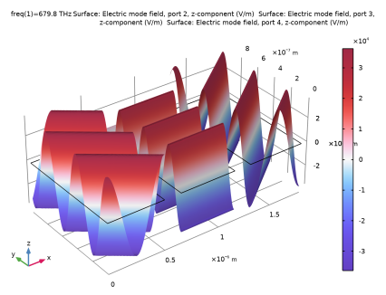
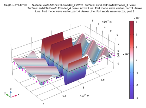
In the Settings window for Surface, click Replace Expression in the upper-right corner of the Expression section. From the menu, choose Component 1 (comp1) > Electromagnetic Waves, Frequency Domain > Ports > Electric mode fields > Electric mode field, port 2 - V/m > ewfd.Emodez_2 - Electric mode field, port 2, z-component. This represents the mode field of the zero-order port on the transmission side.
3
Locate the Coloring and Style section. From the Color table list, choose WaveLight.
4
From the Scale list, choose Linear symmetric.
5
Click to expand the Plot Array section. Select the Manual indexing checkbox.
6
In the Index text field, type 1.
Height Expression 1
Right-click Surface 1 and choose Height Expression.
Surface 2
1
In the Model Builder window, under Results > Diffraction Orders right-click Surface 1 and choose Duplicate.
2
In the Settings window for Surface, locate the Expression section.
3
In the Expression text field, type ewfd.Emodez_3. This is the mode field of diffraction order m = -1 on the transmission side.
4
Click to expand the Inherit Style section. From the Plot list, choose Surface 1.
5
Locate the Plot Array section. In the Index text field, type 0.
Surface 3
1
Right-click Surface 2 and choose Duplicate.
2
In the Settings window for Surface, locate the Expression section.
3
In the Expression text field, type ewfd.Emodez_4. This is the mode field of diffraction order m = 1 on the transmission side.
4
Locate the Plot Array section. In the Index text field, type 2.
5
In the Diffraction Orders toolbar, click  Plot.
6
Click the  Zoom Extents button in the Graphics toolbar.
This plot shows the normalized mode fields. However, it is more instructive to see the mode fields with the correct amplitudes. To do that the mode fields should be multiplied with the S-parameter for the respective port (mode).
Surface 1
1
In the Model Builder window, click Surface 1.
2
In the Settings window for Surface, locate the Expression section.
3
In the Expression text field, type ewfd.S21*ewfd.Emodez_2.
Surface 2
1
In the Model Builder window, click Surface 2.
2
In the Settings window for Surface, locate the Expression section.
3
In the Expression text field, type ewfd.S31*ewfd.Emodez_3.
Surface 3
1
In the Model Builder window, click Surface 3.
2
In the Settings window for Surface, locate the Expression section.
3
In the Expression text field, type ewfd.S41*ewfd.Emodez_4.
4
In the Diffraction Orders toolbar, click  Plot.
5
Click the  Zoom Extents button in the Graphics toolbar.
Diffraction Orders
Add arrows to more clearly show the propagation direction for the different modes.
Arrow Line 1
1
In the Model Builder window, right-click Diffraction Orders and choose Arrow Line.
2
In the Settings window for Arrow Line, click Replace Expression in the upper-right corner of the Expression section. From the menu, choose Component 1 (comp1) > Electromagnetic Waves, Frequency Domain > Ports > Wave vectors > ewfd.kModex_3,ewfd.kModey_3 - Port mode wave vector, port 3.
3
Locate the Arrow Positioning section. In the Number of arrows text field, type 15.
4
Locate the Coloring and Style section. From the Color list, choose Magenta.
5
Click to expand the Plot Array section. Select the Manual indexing checkbox.
Selection 1
1
Right-click Arrow Line 1 and choose Selection.
2
Arrow Line 2
1
In the Model Builder window, under Results > Diffraction Orders right-click Arrow Line 1 and choose Duplicate.
2
In the Settings window for Arrow Line, locate the Expression section.
3
In the X-component text field, type ewfd.kModex_4.
4
In the Y-component text field, type ewfd.kModey_4.
5
Click to expand the Inherit Style section. From the Plot list, choose Arrow Line 1.
6
Locate the Plot Array section. In the Index text field, type 2.
Selection 1
1
In the Model Builder window, expand the Arrow Line 2 node, then click Selection 1.
2
In the Settings window for Selection, locate the Selection section.
3
Click to select the  Activate Selection toggle button.
4
Arrow Line 3
1
In the Model Builder window, under Results > Diffraction Orders right-click Arrow Line 1 and choose Duplicate.
2
In the Settings window for Arrow Line, locate the Expression section.
3
In the X-component text field, type ewfd.kModex_2.
4
In the Y-component text field, type ewfd.kModey_2.
5
Locate the Inherit Style section. From the Plot list, choose Arrow Line 1.
6
Locate the Arrow Positioning section. In the Number of arrows text field, type 5.
7
Locate the Plot Array section. In the Index text field, type 1.
Selection 1
1
In the Model Builder window, expand the Arrow Line 3 node, then click Selection 1.
2
In the Settings window for Selection, locate the Selection section.
3
Click to select the  Activate Selection toggle button.
4
Arrow Line 1
1
In the Model Builder window, under Results > Diffraction Orders click Arrow Line 1.
2
In the Settings window for Arrow Line, locate the Coloring and Style section.
3
Diffraction Orders
1
In the Model Builder window, click Diffraction Orders.
2
In the Diffraction Orders toolbar, click  Plot.
This plot more clearly shows the propagation directions and the amplitudes for the modes on the transmission side.
Animation 1
Finally, add an animation of this plot.
1
In the Diffraction Orders toolbar, click  Animation and choose Player.
2
In the Settings window for Animation, locate the Animation Editing section.
3
From the Sequence type list, choose Dynamic data extension.
4
Locate the Playing section. From the Repeat list, choose Number of iterations.
5
In the Number of iterations text field, type 5.
6
Click the  Play button in the Graphics toolbar.