PDF

Spherical Cap with Central Point Load
Introduction
Buckling is a phenomenon that can cause sudden failure of a structure. A linear buckling analysis predicts the critical buckling load. Such an analysis, however, does not give any information about what happens at loads higher than the critical load. Tracing the solution after the critical load is called a postbuckling analysis.
A spherical cap with a point load at its crown is a common example to study postbuckling analysis of 2D axisymmetric shells. The critical load, snap-through behavior, and softening and stiffening effects are the interesting aspects which are studied in this example.
In order to predict the postbuckling behavior, one need to use the nonlinear solver and ramp up the applied load to compute the structure deformation. The buckling load can then be based on when a certain, not acceptable, deformation is reached.
Once the critical buckling load has been reached, it can happen that the structure undergoes a sudden large deformation into a new stable configuration. This is known as a snap-through phenomenon. A snap-through phenomenon cannot be always simulated using prescribed load in a standard nonlinear static solver because the problem becomes numerically singular. In the current example, the displacement at the crown increases monotonically even if the load decreases after a critical point in the snap-through region. Thus, using displacement control is a useful strategy for this example.
Model Definition
The model studied here is a benchmark for a spherical cap subjected to a point load at its crown; see Ref. 1.
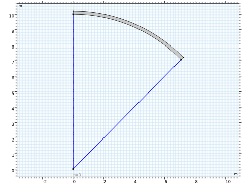
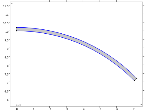
The radius of the spherical cap is a = 10 m and the thickness is th = 0.20384 m. The sector angle of the spherical cap is π/4 radians.
Due to the axial symmetry, only the part of the cap which is located at positive r-coordinates is modeled. The full geometry of the spherical cap with loading and boundary conditions is shown in Figure 1.
Figure 1: Problem description.
Results
For a spherical cap, the load versus displacement curve exhibits a critical load which is followed by a gradual snap and further increase in stiffness. Figure 2 and Figure 3 show the total displacement using the Solid Mechanics and Shell interfaces, respectively, at three different crown displacements. The annotations in the figures shows the corresponding point loads which closely match the benchmarked numerical solutions given in Ref. 1.
Figure 2: Total displacement computed in the Solid Mechanics Interface using 40 mesh elements.
What is important to note in the figures is the snap-through behavior and softening effect after the critical load. The top surface in both figures corresponds to the critical load, while the middle surface is corresponding to the load after the critical point. This shows that although deformation increases, the load decreases due to softening after the critical load. The third surface in both figures shows an increase in displacement with an increase in load, indicating an increase in stiffness after the snap through phase.
Figure 4 shows the variation of axial displacement at the crown of the spherical cap versus the applied load. For the Shell interface, three different discretizations (4, 8, 16 mesh elements) are used. For the Solid Mechanics interface 40 mesh elements are used. These discretizations are the same as in Ref. 1.
The results match the values in the reference quite closely. Note however, that these results are reported for certain discretizations and element formulations. There is no target value as such.
Figure 3: Total displacement computing in the Shell Interface using 16 mesh elements.
Figure 4: Applied load versus center displacement.
In Table 1, the results from the Solid Mechanics interface with 40 mesh elements are compared with the reference.
In Table 2, Table 3, and Table 4, the results from the Shell interface with 4, 8, and 16 mesh elements, respectively, are compared with the reference. Note that with only four elements, there is no snap through behavior, indicating that the mesh is much too coarse. This is experienced also in the reference, even though different types of shell element formulations are used.
Note that the lowest load after the critical load when using a shell formulation is 1.678 in the reference. This value is not reached in the solutions, where the lowest load is predicted as 1.722 and 1.717 with 8 and 16 elements, respectively. A refined Solid Mechanics model actually indicates that the current values computed here are more accurate than those reported in the reference.
Notes About the COMSOL Implementation
The main feature of this model is that a limit point instability occurs at the buckling load. Load control would not able to track the unstable solution paths after the limit point, so a displacement control is used since the displacement at the crown increases monotonically.
In this case, where the only load is a point load, it would be possible to directly prescribe the displacement in that point, and then measure the reaction force. If the load was more complex, for example a pressure load, that would not be possible. For this reason, a more general approach is shown here.
To employ a displacement control strategy, a point load at the crown is considered as a global degree of freedom and a global equation in terms of axial displacement at the crown is solved to get the point load value.
For a nonlinear problem experiencing a snap-through behavior, there is no general way to determine which controlling parameter to use, so it is necessary to use some physical insight. You need to find a quantity which is monotonically increasing to use as a controlling parameter.
Reference
1. P. Lyons and S. Holsgrove, Finite Element Benchmarks For 2D Beams And Axisymmetric Shells Involving Geometric Non-Linearity, NAFEMS, 2005.
Application Library path: Structural_Mechanics_Module/Verification_Examples/spherical_cap_with_central_point_load
Modeling Instructions
From the File menu, choose New.
New
In the New window, click  Model Wizard.
Model Wizard
1
In the Model Wizard window, click  2D Axisymmetric.
2
In the Select Physics tree, select Structural Mechanics > Solid Mechanics (solid).
3
Click Add.
4
In the Select Physics tree, select Structural Mechanics > Shell (shell).
5
Click Add.
6
Global Definitions
Parameters 1
1
In the Model Builder window, under Global Definitions click Parameters 1.
2
In the Settings window for Parameters, locate the Parameters section.
3
Define a set of nondimensional variables that will be useful in the postprocessing plots and evaluations.
Definitions
Variables 1
1
In the Model Builder window, under Component 1 (comp1) right-click Definitions and choose Variables.
2
In the Settings window for Variables, locate the Variables section.
3
Geometry 1
Circle 1 (c1)
1
In the Geometry toolbar, click  Circle.
2
In the Settings window for Circle, locate the Object Type section.
3
From the Type list, choose Curve.
4
Locate the Size and Shape section. In the Sector angle text field, type 45.
5
In the Radius text field, type a+th.
6
Click  Build Selected.
7
Locate the Rotation Angle section. In the Rotation text field, type 45.
8
Click to expand the Layers section. In the table, enter the following settings:
9
Click  Build Selected.
Delete Entities 1 (del1)
1
In the Model Builder window, right-click Geometry 1 and choose Delete Entities.
2
On the object c1, select Boundaries 1 and 2 only.
3
Click the  Zoom Extents button in the Graphics toolbar.
4
In the Settings window for Delete Entities, click  Build Selected.
Use the same material through a material link for the Solid Mechanics and Shell interfaces.
Global Definitions
Material 1 (mat1)
In the Model Builder window, under Global Definitions right-click Materials and choose Blank Material.
Materials
Material Link 1 (matlnk1)
In the Model Builder window, under Component 1 (comp1) right-click Materials and choose More Materials > Material Link.
Material Link 2 (matlnk2)
1
Right-click Materials and choose More Materials > Material Link.
2
In the Settings window for Material Link, locate the Geometric Entity Selection section.
3
From the Geometric entity level list, choose Boundary.
4
It might be easier to select the correct boundary by using the Selection List window. To open this window, in the Home toolbar click Windows and choose Selection List. (If you are running the cross-platform desktop, you find Windows in the main menu.)
Global Definitions
Material 1 (mat1)
1
In the Model Builder window, under Global Definitions > Materials click Material 1 (mat1).
2
In the Settings window for Material, locate the Material Contents section.
3
Definitions
Integration 1 (intop1)
1
In the Definitions toolbar, click  Nonlocal Couplings and choose Integration.
2
In the Settings window for Integration, locate the Source Selection section.
3
From the Geometric entity level list, choose Point.
4
5
Locate the Advanced section. From the Method list, choose Summation over nodes.
Solid Mechanics (solid)
Fixed Constraint 1
1
In the Physics toolbar, click  Boundaries and choose Fixed Constraint.
2
Now add a global equation for a point load, so that the crown displacement equals the prescribed one. For that, you need to show equation-based contributions.
3
Click the  Show More Options button in the Model Builder toolbar.
4
In the Show More Options dialog, in the tree, select the checkbox for the node Physics > Equation-Based Contributions.
5
Global Equations 1 (ODE1)
1
In the Physics toolbar, click  Global and choose Global Equations.
2
In the Settings window for Global Equations, locate the Global Equations section.
3
4
Locate the Units section. Click  Select Dependent Variable Quantity.
5
In the Physical Quantity dialog, type force in the text field.
6
In the tree, select General > Force (N).
7
8
In the Settings window for Global Equations, locate the Units section.
9
Click  Select Source Term Quantity.
10
In the Physical Quantity dialog, type disp in the text field.
11
In the tree, select General > Displacement (m).
12
Point Load (on Axis) 1
1
In the Physics toolbar, click  Points and choose Point Load (on Axis).
2
3
In the Settings window for Point Load (on Axis), locate the Force section.
4
From the Fz list, choose State variable F1 (solid).
Shell (shell)
1
In the Model Builder window, under Component 1 (comp1) click Shell (shell).
2
In the Settings window for Shell, locate the Boundary Selection section.
3
Click  Clear Selection.
4
In order to model the solid midplane using the Shell interface, assign a proper offset from the Thickness and Offset feature. The shell normal is pointing inward which can be verified in the postprocessing plot.
Thickness and Offset 1
1
In the Model Builder window, under Component 1 (comp1) > Shell (shell) click Thickness and Offset 1.
2
In the Settings window for Thickness and Offset, locate the Thickness and Offset section.
3
In the d0 text field, type th.
4
From the Position list, choose Top surface on boundary.
Fixed Constraint 1
1
In the Physics toolbar, click  Points and choose Fixed Constraint.
2
Global Equations 1 (ODE2)
1
In the Physics toolbar, click  Global and choose Global Equations.
2
In the Settings window for Global Equations, locate the Global Equations section.
3
4
Locate the Units section. Click  Select Dependent Variable Quantity.
5
In the Physical Quantity dialog, type force in the text field.
6
In the tree, select General > Force (N).
7
8
In the Settings window for Global Equations, locate the Units section.
9
Click  Select Source Term Quantity.
10
In the Physical Quantity dialog, type disp in the text field.
11
In the tree, select General > Displacement (m).
12
Point Load (on Axis) 1
1
In the Physics toolbar, click  Points and choose Point Load (on Axis).
2
3
In the Settings window for Point Load (on Axis), locate the Force section.
4
From the Fz list, choose State variable F2 (shell).
Use different Mesh nodes in order to use different discretizations for Solid Mechanics and Shell interfaces as given in the benchmark example.
Mesh 2
In the Mesh toolbar, click Add Mesh and choose Add Mesh.
Mesh: Solid Mechanics
1
In the Model Builder window, under Component 1 (comp1) > Meshes click Mesh 1.
2
In the Settings window for Mesh, type Mesh: Solid Mechanics in the Label text field.
Mapped 1
In the Mesh toolbar, click  Mapped.
Distribution 1
1
Right-click Mapped 1 and choose Distribution.
2
3
In the Settings window for Distribution, locate the Distribution section.
4
In the Number of elements text field, type 40.
5
Click  Build Selected.
Mesh: Shell
1
In the Model Builder window, under Component 1 (comp1) > Meshes click Mesh 2.
2
In the Settings window for Mesh, type Mesh: Shell in the Label text field.
Edge 1
1
In the Mesh toolbar, click  More Generators and choose Edge.
2
Distribution 1
1
Right-click Edge 1 and choose Distribution.
2
In the Settings window for Distribution, locate the Distribution section.
3
In the Number of elements text field, type meshdist.
4
Click  Build Selected.
Add a stationary study to the Solid Mechanics interface.
Add Study
1
In the Home toolbar, click  Add Study to open the Add Study window.
2
Go to the Add Study window.
3
Find the Studies subsection. In the Select Study tree, select General Studies > Stationary.
4
Find the Physics interfaces in study subsection. In the table, clear the Solve checkbox for Shell (shell).
5
Click the Add Study button in the window toolbar.
6
In the Home toolbar, click  Add Study to close the Add Study window.
Study: Solid Mechanics
In the Settings window for Study, type Study: Solid Mechanics in the Label text field.
Step 1: Stationary
1
In the Model Builder window, under Study: Solid Mechanics click Step 1: Stationary.
2
In the Settings window for Stationary, locate the Study Settings section.
3
Select the Include geometric nonlinearity checkbox.
4
Click to expand the Mesh Selection section. In the table, enter the following settings:
5
Click to expand the Study Extensions section. Select the Auxiliary sweep checkbox.
6
7
8
In the Study toolbar, click  Compute.
Add a stationary study to the Shell interface. Parameterize the mesh discretization using a parametric sweep.
Add Study
1
In the Home toolbar, click  Add Study to open the Add Study window.
2
Go to the Add Study window.
3
Find the Studies subsection. In the Select Study tree, select General Studies > Stationary.
4
Find the Physics interfaces in study subsection. In the table, clear the Solve checkbox for Solid Mechanics (solid).
5
Click the Add Study button in the window toolbar.
6
In the Home toolbar, click  Add Study to close the Add Study window.
Study: Shell
In the Settings window for Study, type Study: Shell in the Label text field.
Parametric Sweep
1
In the Study toolbar, click  Parametric Sweep.
2
In the Settings window for Parametric Sweep, locate the Study Settings section.
3
4
Step 1: Stationary
1
In the Model Builder window, click Step 1: Stationary.
2
In the Settings window for Stationary, locate the Study Settings section.
3
Select the Include geometric nonlinearity checkbox.
4
Locate the Study Extensions section. Select the Auxiliary sweep checkbox.
5
6
7
In the Study toolbar, click  Compute.
Results
Revolution 2D
1
In the Model Builder window, expand the Results > Datasets node, then click Revolution 2D.
2
In the Settings window for Revolution 2D, click to expand the Revolution Layers section.
3
In the Start angle text field, type 45.
4
In the Revolution angle text field, type -90.
Revolution 2D 2
1
In the Model Builder window, click Revolution 2D 2.
2
In the Settings window for Revolution 2D, locate the Revolution Layers section.
3
In the Start angle text field, type 45.
4
In the Revolution angle text field, type -90.
Stress (solid)
1
In the Model Builder window, under Results click Stress (solid).
2
In the Settings window for 2D Plot Group, locate the Plot Settings section.
3
From the Frame list, choose Material  (R, PHI, Z).
In order to visualize the softening and stiffening effect after the critical point, generate a 3D displacement plot of the spherical cap at the critical point, and on the unstable and stable part of the equilibrium path after the critical point.
Total Displacement, 3D (solid)
1
In the Model Builder window, under Results click Stress, 3D (solid).
2
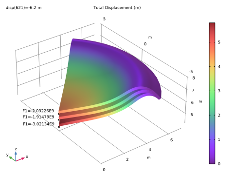
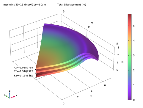
In the Settings window for 3D Plot Group, type Total Displacement, 3D (solid) in the Label text field.
3
Click to expand the Title section. From the Title type list, choose Manual.
4
In the Title text area, type Total Displacement (m).
5
Locate the Plot Settings section. Clear the Plot dataset edges checkbox.
Surface 1
1
In the Model Builder window, expand the Total Displacement, 3D (solid) node, then click Surface 1.
2
In the Settings window for Surface, locate the Data section.
3
From the Dataset list, choose Revolution 2D.
4
From the Parameter value (disp (m)) list, choose -4.7.
5
Locate the Expression section. In the Expression text field, type solid.disp.
6
Locate the Coloring and Style section. From the Color table list, choose SpectrumLight.
Annotation 1
1
In the Model Builder window, expand the Surface 1 node.
2
Right-click Total Displacement, 3D (solid) and choose Annotation.
3
In the Settings window for Annotation, locate the Data section.
4
From the Dataset list, choose Revolution 2D.
5
From the Parameter value (disp (m)) list, choose -4.7.
6
Locate the Annotation section. In the Text text field, type F1=eval(F1).
7
From the Geometry level list, choose Global.
8
Locate the Position section. In the Z text field, type a-4.7.
9
Click to expand the Advanced section. Locate the Coloring and Style section. From the Anchor point list, choose Lower right.
Surface 2
In the Model Builder window, under Results > Total Displacement, 3D (solid) right-click Surface 1 and choose Duplicate.
Annotation 2
In the Model Builder window, under Results > Total Displacement, 3D (solid) right-click Annotation 1 and choose Duplicate.
Surface 2
1
In the Settings window for Surface, locate the Data section.
2
From the Parameter value (disp (m)) list, choose -5.2.
3
Click to expand the Inherit Style section. From the Plot list, choose Surface 1.
Annotation 2
1
In the Model Builder window, click Annotation 2.
2
In the Settings window for Annotation, locate the Data section.
3
From the Parameter value (disp (m)) list, choose -5.2.
4
Locate the Position section. In the Z text field, type a-5.2.
Surface 3
In the Model Builder window, under Results > Total Displacement, 3D (solid) right-click Surface 2 and choose Duplicate.
Annotation 3
In the Model Builder window, under Results > Total Displacement, 3D (solid) right-click Annotation 2 and choose Duplicate.
Surface 3
1
In the Settings window for Surface, locate the Data section.
2
From the Parameter value (disp (m)) list, choose -5.8.
Annotation 3
1
In the Model Builder window, click Annotation 3.
2
In the Settings window for Annotation, locate the Data section.
3
From the Parameter value (disp (m)) list, choose -5.8.
4
Locate the Position section. In the Z text field, type a-5.8.
5
In the Total Displacement, 3D (solid) toolbar, click  Plot.
6
Click the  Zoom Extents button in the Graphics toolbar.
Stress (shell)
1
In the Model Builder window, under Results click Stress (shell).
2
In the Settings window for 2D Plot Group, locate the Plot Settings section.
3
From the Frame list, choose Material  (R, PHI, Z).
Total Displacement, 3D (shell)
1
In the Model Builder window, under Results click Stress, 3D (shell).
2
In the Settings window for 3D Plot Group, type Total Displacement, 3D (shell) in the Label text field.
3
Locate the Title section. From the Title type list, choose Manual.
4
In the Title text area, type Total Displacement (m).
5
Locate the Plot Settings section. Clear the Plot dataset edges checkbox.
Surface 1
1
In the Model Builder window, expand the Total Displacement, 3D (shell) node, then click Surface 1.
2
In the Settings window for Surface, locate the Data section.
3
From the Dataset list, choose Revolution 2D 2.
4
From the Parameter value (disp (m)) list, choose -4.7.
5
Locate the Expression section. In the Expression text field, type shell.disp.
6
Locate the Coloring and Style section. From the Color table list, choose SpectrumLight.
Annotation 1
1
In the Model Builder window, expand the Surface 1 node.
2
Right-click Total Displacement, 3D (shell) and choose Annotation.
3
In the Settings window for Annotation, locate the Data section.
4
From the Dataset list, choose Revolution 2D 2.
5
From the Parameter value (disp (m)) list, choose -4.7.
6
Locate the Annotation section. In the Text text field, type F2=eval(F2).
7
From the Geometry level list, choose Global.
8
Locate the Position section. In the z text field, type a-4.7.
9
Locate the Coloring and Style section. From the Anchor point list, choose Lower right.
Surface 2
In the Model Builder window, under Results > Total Displacement, 3D (shell) right-click Surface 1 and choose Duplicate.
Annotation 2
In the Model Builder window, under Results > Total Displacement, 3D (shell) right-click Annotation 1 and choose Duplicate.
Surface 2
1
In the Settings window for Surface, locate the Data section.
2
From the Parameter value (disp (m)) list, choose -5.2.
3
Locate the Inherit Style section. From the Plot list, choose Surface 1.
Annotation 2
1
In the Model Builder window, click Annotation 2.
2
In the Settings window for Annotation, locate the Data section.
3
From the Parameter value (disp (m)) list, choose -5.2.
4
Locate the Position section. In the z text field, type a-5.2.
Surface 3
In the Model Builder window, under Results > Total Displacement, 3D (shell) right-click Surface 2 and choose Duplicate.
Annotation 3
In the Model Builder window, under Results > Total Displacement, 3D (shell) right-click Annotation 2 and choose Duplicate.
Surface 3
1
In the Settings window for Surface, locate the Data section.
2
From the Parameter value (disp (m)) list, choose -5.8.
Annotation 3
1
In the Model Builder window, click Annotation 3.
2
In the Settings window for Annotation, locate the Data section.
3
From the Parameter value (disp (m)) list, choose -5.8.
4
Locate the Position section. In the z text field, type a-5.8.
5
In the Total Displacement, 3D (shell) toolbar, click  Plot.
6
Click the  Zoom Extents button in the Graphics toolbar.
Visualize the shell thickness and normal orientation.
Result Templates
1
In the Results toolbar, click  Result Templates to open the Result Templates window.
2
Go to the Result Templates window.
3
In the tree, select Study: Shell/Parametric Solutions 1 (sol3) > Shell > Thickness and Orientation (shell).
4
Click the Add Result Template button in the window toolbar.
5
In the Results toolbar, click  Result Templates to close the Result Templates window.
Results
Thickness and Orientation (shell)
In order to better visualize the shell normal in the Thickness and Orientation plot, reduce the number of arrows.
Shell Local System
1
In the Model Builder window, expand the Thickness and Orientation (shell) node, then click Shell Local System.
2
In the Settings window for Coordinate System Line, locate the Positioning section.
3
In the Number of points text field, type 20.
4
In the Thickness and Orientation (shell) toolbar, click  Plot.
Plot a 1D curve showing the relationship between the axial displacement and the point load at the crown.
Load vs. Displacement at Crown
1
In the Results toolbar, click  1D Plot Group.
2
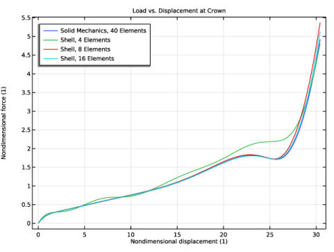
In the Settings window for 1D Plot Group, type Load vs. Displacement at Crown in the Label text field.
3
Click to expand the Title section. From the Title type list, choose Manual.
4
In the Title text area, type Load vs. Displacement at Crown.
5
Locate the Legend section. From the Position list, choose Upper left.
Point Graph 1
1
Right-click Load vs. Displacement at Crown and choose Point Graph.
2
3
In the Settings window for Point Graph, locate the y-Axis Data section.
4
In the Expression text field, type Fn1.
5
Locate the x-Axis Data section. From the Parameter list, choose Expression.
6
In the Expression text field, type wn1.
7
Click to expand the Legends section. Select the Show legends checkbox.
8
From the Legends list, choose Manual.
9
Point Graph 2
1
Right-click Point Graph 1 and choose Duplicate.
2
In the Settings window for Point Graph, locate the Data section.
3
From the Dataset list, choose Study: Shell/Parametric Solutions 1 (sol3).
4
Locate the y-Axis Data section. In the Expression text field, type Fn2.
5
Locate the x-Axis Data section. In the Expression text field, type wn2.
6
Locate the Legends section. From the Legends list, choose Evaluated.
7
In the Legend text field, type Shell, eval(meshdist) Elements.
8
In the Load vs. Displacement at Crown toolbar, click  Plot.
Load vs. Displacement at Crown
1
In the Results toolbar, click  Evaluation Group.
2
In the Settings window for Evaluation Group, type Load vs. Displacement at Crown in the Label text field.
Solid Mechanics, 40 Elements
1
Right-click Load vs. Displacement at Crown and choose Point Evaluation.
2
In the Settings window for Point Evaluation, type Solid Mechanics, 40 Elements in the Label text field.
3
Locate the Data section. From the Dataset list, choose Study: Solid Mechanics/Solution 1 (sol1).
4
5
Locate the Expressions section. In the table, enter the following settings:
Shell, 4 Elements
1
In the Model Builder window, right-click Load vs. Displacement at Crown and choose Point Evaluation.
2
In the Settings window for Point Evaluation, type Shell, 4 Elements in the Label text field.
3
Locate the Data section. From the Dataset list, choose Study: Shell/Parametric Solutions 1 (sol3).
4
From the Parameter selection (meshdist) list, choose From list.
5
In the Parameter values (meshdist) list, select 4.
6
7
Locate the Expressions section. In the table, enter the following settings:
Shell, 8 Elements
1
Right-click Shell, 4 Elements and choose Duplicate.
2
In the Settings window for Point Evaluation, type Shell, 8 Elements in the Label text field.
3
Locate the Data section. In the Parameter values (meshdist) list, select 8.
4
Locate the Expressions section. In the table, enter the following settings:
Shell, 16 Elements
1
Right-click Shell, 8 Elements and choose Duplicate.
2
In the Settings window for Point Evaluation, type Shell, 16 Elements in the Label text field.
3
Locate the Data section. In the Parameter values (meshdist) list, select 16.
4
Locate the Expressions section. In the table, enter the following settings:
Load vs. Displacement at Crown
1
In the Model Builder window, click Load vs. Displacement at Crown.
2
In the Settings window for Evaluation Group, click to expand the Format section.
3
From the Include parameters list, choose Off.
4
In the Load vs. Displacement at Crown toolbar, click  Evaluate.