|
|
|
|
•
|
|
•
|
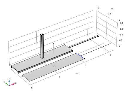
Plate thickness: 10 mm
|
|
•
|
|
•
|
|
•
|
|
•
|
|
•
|
|
•
|
A uniform pressure of 5 kPa is applied to the top of the plate.
|
|
•
|
|
•
|
|
•
|
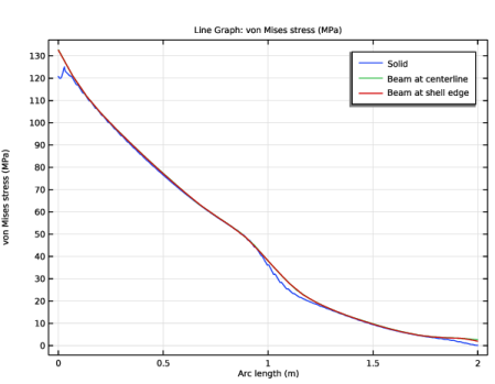
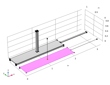
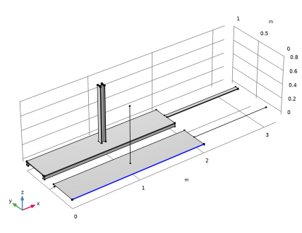
The longitudinal stiffening beams are connected to the long edges of the plate. Two different modeling possibilities are used. On one side, there is a separate edge at the center of the beam (Figure 6), whereas on the other side, the edge of the shell is also used for the beam (Figure 5), and the actual location of the beam is specified using the offset property in the settings for Shell-Beam Connection.
|
|
•
|
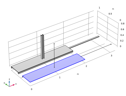
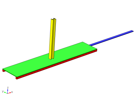
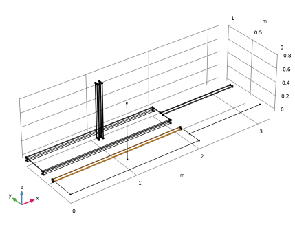
The H-section beam is perpendicular to the plate (Figure 7). The endpoint of it is connected to a representative region on the shell surface, using a Boolean expression that is a function of the coordinates. This expression makes the connection act on a 70-by-60 mm rectangular area centered around the end of the beam. You could easily modify that expression so that only the actual H-shape is connected, possibly allowing for a weld thickness. Another option could be use a pure distance criterion, where a circle with a given diameter is connected.
|
|
•
|
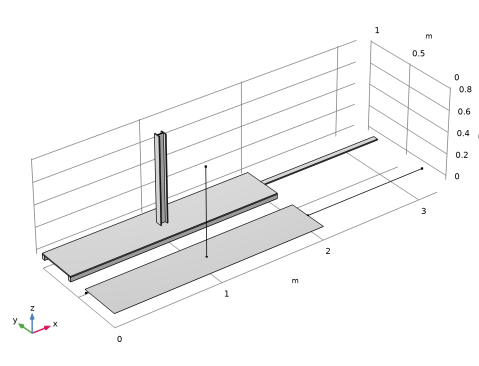
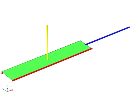
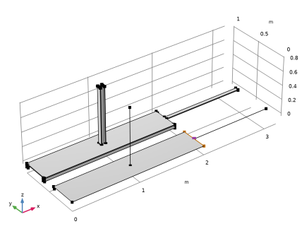
The central beam is modeled as a beam only for instructional purposes. In practice it would be simpler to treat it as an extension of the plate. This beam has its endpoint connected to the edge of the shell (Figure 8). The part of the edge which is connected is selected as the width of the beam.
 |
|
1
|
|
2
|
|
3
|
Click Add.
|
|
4
|
|
5
|
Click Add.
|
|
6
|
|
7
|
Click Add.
|
|
8
|
Click
|
|
9
|
|
10
|
Click
|
|
1
|
|
2
|
|
3
|
Click
|
|
4
|
Browse to the model’s Application Libraries folder and double-click the file shell_beam_connection_parameters.txt.
|
|
1
|
|
2
|
|
3
|
|
4
|
|
5
|
|
1
|
|
2
|
|
3
|
|
4
|
|
5
|
|
6
|
|
7
|
Click
|
|
1
|
|
2
|
|
3
|
|
4
|
Click
|
|
1
|
|
2
|
|
3
|
|
4
|
|
5
|
|
6
|
|
7
|
|
8
|
Click
|
|
1
|
|
2
|
|
3
|
|
4
|
Click
|
|
1
|
|
2
|
|
3
|
|
4
|
|
5
|
|
6
|
|
7
|
|
8
|
|
1
|
|
2
|
|
3
|
|
4
|
|
5
|
|
6
|
|
7
|
|
8
|
|
1
|
Right-click Component 1 (comp1) > Geometry 1 > Work Plane 1 (wp1) > Plane Geometry > Rectangle 2 (r2) and choose Duplicate.
|
|
2
|
|
3
|
|
4
|
|
1
|
In the Model Builder window, under Component 1 (comp1) > Geometry 1 right-click Work Plane 1 (wp1) and choose Extrude.
|
|
2
|
|
4
|
Click
|
|
1
|
|
2
|
Click in the Graphics window and then press Ctrl+A to select all objects.
|
|
3
|
|
4
|
|
5
|
Click
|
|
1
|
|
2
|
|
1
|
|
2
|
|
3
|
|
4
|
|
5
|
|
1
|
|
2
|
|
4
|
Click
|
|
1
|
|
2
|
|
4
|
Click
|
|
1
|
|
2
|
|
4
|
Click
|
|
1
|
|
2
|
|
3
|
|
4
|
|
1
|
|
2
|
|
3
|
|
4
|
On the object pol3, select Edge 1 only.
|
|
5
|
|
6
|
|
7
|
Click OK.
|
|
1
|
|
2
|
|
3
|
|
4
|
On the object pol2, select Edge 1 only.
|
|
5
|
On the object wp2, select Edge 1 only.
|
|
6
|
Locate the Resulting Selection section. Find the Cumulative selection subsection. From the Contribute to list, choose Beam.
|
|
1
|
|
2
|
|
3
|
|
4
|
On the object pol1, select Edge 1 only.
|
|
5
|
Locate the Resulting Selection section. Find the Cumulative selection subsection. From the Contribute to list, choose Beam.
|
|
6
|
|
7
|
|
1
|
|
2
|
Go to the Add Material window.
|
|
3
|
|
4
|
Click the right end of the Add to Component split button in the window toolbar.
|
|
5
|
From the menu, choose Add to Global Materials.
|
|
6
|
|
1
|
|
2
|
|
3
|
|
4
|
|
1
|
|
2
|
|
3
|
|
4
|
|
1
|
|
1
|
|
3
|
|
4
|
|
5
|
|
1
|
|
3
|
|
4
|
|
5
|
|
1
|
|
3
|
|
4
|
|
1
|
|
2
|
|
3
|
Click
|
|
4
|
|
1
|
In the Model Builder window, under Component 1 (comp1) > Shell (shell) click Thickness and Offset 1.
|
|
2
|
|
3
|
|
1
|
|
1
|
|
2
|
|
3
|
|
4
|
|
1
|
|
2
|
|
3
|
Click
|
|
4
|
|
1
|
|
2
|
|
3
|
|
4
|
|
5
|
|
1
|
|
2
|
|
3
|
|
4
|
Specify the V vector as
|
|
1
|
|
2
|
|
3
|
|
4
|
|
5
|
|
6
|
|
7
|
|
8
|
|
1
|
|
2
|
|
3
|
|
4
|
Specify the V vector as
|
|
1
|
|
2
|
|
3
|
|
4
|
|
5
|
|
6
|
|
1
|
|
2
|
|
3
|
|
4
|
Specify the V vector as
|
|
1
|
|
3
|
|
4
|
|
1
|
|
3
|
|
4
|
|
5
|
|
1
|
|
2
|
|
3
|
|
4
|
Select the Manual control of selections checkbox.
|
|
5
|
|
7
|
|
8
|
|
1
|
|
2
|
|
3
|
|
4
|
|
6
|
|
8
|
Click to clear the
|
|
9
|
|
10
|
|
1
|
|
2
|
|
3
|
|
4
|
Select the Manual control of selections checkbox.
|
|
5
|
|
7
|
|
9
|
Click to clear the
|
|
10
|
Locate the Connection Settings section. From the Connected region list, choose Connection criterion.
|
|
11
|
In the text field, type (abs(x-lp/2)<hbh/2)*(abs(y-wp/2)<wbh/2).
|
|
1
|
|
2
|
|
3
|
Select the Manual control of selections checkbox.
|
|
4
|
|
6
|
|
7
|
Click
|
|
9
|
Click to clear the
|
|
10
|
|
11
|
|
1
|
|
1
|
|
3
|
|
4
|
|
1
|
|
3
|
|
4
|
Click the Custom button.
|
|
5
|
Locate the Element Size Parameters section.
|
|
6
|
|
1
|
|
1
|
|
2
|
|
3
|
|
5
|
|
6
|
Locate the Element Size Parameters section.
|
|
7
|
|
8
|
|
1
|
|
2
|
|
3
|
|
4
|
Click
|
|
1
|
|
2
|
|
3
|
|
4
|
Click
|
|
1
|
|
2
|
|
3
|
In the Model Builder window, expand the Study 1 > Solver Configurations > Solution 1 (sol1) > Stationary Solver 1 node.
|
|
4
|
Right-click Study 1 > Solver Configurations > Solution 1 (sol1) > Stationary Solver 1 and choose Fully Coupled.
|
|
5
|
|
1
|
|
2
|
|
3
|
Click
|
|
4
|
|
5
|
Click OK.
|
|
6
|
|
8
|
Click
|
|
1
|
|
2
|
|
1
|
|
2
|
|
3
|
|
1
|
|
2
|
|
3
|
|
4
|
|
1
|
|
2
|
|
3
|
|
1
|
|
2
|
|
3
|
Clear the Show grid checkbox.
|
|
1
|
|
2
|
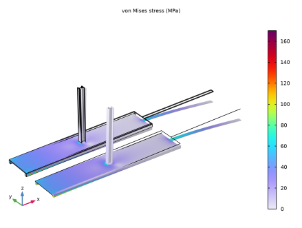
In the Settings window for 3D Plot Group, type Stress (solid, shell and beam) in the Label text field.
|
|
3
|
|
4
|
|
5
|
|
6
|
|
1
|
|
2
|
|
1
|
|
3
|
|
4
|
|
5
|
|
6
|
|
1
|
|
3
|
|
4
|
|
5
|
|
6
|
|
7
|
|
8
|
|
1
|
|
2
|
|
3
|
Click
|
|
5
|
Locate the Legends section. In the table, enter the following settings:
|
|
6
|