COMSOL 6.3 - Postbuckling Analysis of an Aircraft Fuselage

Postbuckling Analysis of an Aircraft Fuselage

In this model, an aircraft fuselage structure made of a skin–stringer assembly connected by rivets is studied. Frames and stringers reinforce the structure in the hoop and axial directions, respectively. In the case of compressive axial forces, such a lightweight structure can be subject to failure due to local buckling.

A postbuckling analysis of the structure is performed. An important part of this example is to show how to use the feature to connect boundaries in the Shell interface.

Model Definition

The full geometry consists of C-shape frames connected with U-shape stringers and surrounded by a 1 mm thick skin sheet. All parts of the assembly are made of aluminum. The diameter of the fuselage is 4 m.

The frames have a 0.5 m spacing in the longitudinal direction and there are 60 stringers in the circumferential direction. The beams, made of aluminum, have dimensions 60 mm by 20 mm for the frames, and 30 mm by 20 mm for the stringers. Both have the thickness 1.3 mm.

All parts of the assembly are joined using steel rivets with a diameter of 6 mm. For the skin–stringer connection, the rivet pitch is chosen to be 50 mm to avoid inter-rivet buckling. The rivet holes are represented in the geometry.

A 15 mm high L-shape clip is used for the connection between the frame and the stringers.

The model geometry is a section of the full geometry including two frame segments and two stringers. As shown in Figure 1, the section cut is 1 m long and 1/30th in the circumferential direction.

Figure 1: Model geometry of an aircraft fuselage panel.

The rivets connect all parts by transmitting normal and tangential forces. When buckling occurs, it is important to also include contact forces to avoid that parts overlap away from the rivet holes.

The fuselage skin is pressurized at p = 0.5 atm. In an ideal cylinder with radius R and thickness t, this pressure generates an axial stress (σa) and a hoop stress (σh) with the relation

(1)

In the current geometry, the force is shared between the skin and the stiffening elements, but the same relation applies between the resultant circumferential and axial forces.

In the axial direction, an additional compressive load is added to study the structure when buckling occurs. The relation between the axial force, Fa, and the force in the hoop direction, Fh, is then

(2):

where Aa and Ah are the areas in the axial and hoop directions, respectively, and k is a biaxial loading parameter varying from −0.5 (nominal pressure condition) to 1 (compressive loading condition).

The edges in the plane normal to the hoop direction are constrained using symmetry conditions.

The edges in the plane normal to the axial direction are also given symmetry conditions. On one side, a standard symmetry condition is used, while on the opposite side the normal displacement is constant but nonzero. Instead, the axial force is prescribed, using the axial force Fa from Equation 2.

The following safety criterion is evaluated to check whether or not the rivets can sustain the transmitted force:

(3)

Here, Fn,max is the critical normal force defined as function of the rivet yield stress σ0 and rivet diameter d as

(4)

The form of Equation 3 essentially implies a Tresca yield criterion for the rivets.

The mesh size is set with a maximum element size of 10 mm, and a minimum element size of 3 mm, giving the mesh shown in Figure 2.

Figure 2: Model mesh.

With the chosen element size, there are at least eight elements around the each rivet hole.

Results and Discussion

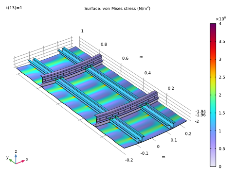
Figure 3 below shows the von Mises stress for the fully compressive loading case. The pattern clearly shows the buckling in the skin. Note that high stress values occur around the rivet holes. This is because the forces between the joined plates are transmitted by the hole edges. The stress at some distance away from a rivet hole is, however, not affected by this local singularity.

Figure 3: von Mises Stress under compressive loading.

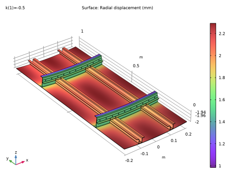
Figure 4 shows the displacement in the radial direction for the nominal pressure loading condition. The stiffening effect of the stringers is clearly visible.

Figure 4: Radial displacement at nominal pressure.

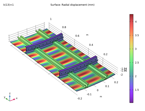
Figure 5 shows the radial displacement at maximum compressive load when the skin has started to buckle.

Figure 5: Radial displacement after buckling.

Figure 6 shows the axial displacement variation with respect to the biaxial loading parameter. For the nominal pressure condition (on the left), the axial displacement is positive and slightly decrease as the compressive axial force increase. Around 0.6 the slope of the curve changes since buckling occurs.

Figure 6: Axial displacement versus biaxial loading parameter.

Figure 7 shows the contact pressure at the frame–stringer intersection under maximum compressive loading.

Figure 7: Contact pressure.

Notes About the COMSOL Implementation

The feature is intended to model ideal local joint connection between two shell boundaries. The axial, shear, and bending forces transmitted by the fasteners are directly applied at the edges of the connected fastener holes. By default, the fastener flexibilities are evaluated based on a beam idealization. They can be tuned by the user. Alternatively, you can provide user-defined normal and tangential stiffness values.

Once the solution is available, you can visualize and evaluate the fastener forces by using result templates for plots and evaluation groups. Figure 8 shows some of the forces acting on the rivets. The tangential forces are shown in blue and the axial forces in green. An annotation is included for each fastener to make them easily identifiable. In Figure 8, the rivets with the highest tangential forces are marked with 5 (fst2) and 7 (fst2). This should be interpreted as the fasteners with number 5 and 7, respectively, defined in the node with the tag fst2. In the evaluation group you can find the values, which are about 860 N.

Figure 8: Forces acting on rivets for the compressive loading case.

If a subnode has been added to a node, the arrows are colored red for fasteners that do not satisfy the safety criterion.

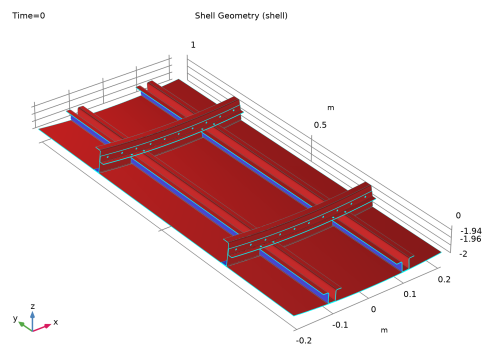
As shell elements are defined on embedded faces in 3D, there is no geometric distinction between the physical top and bottom surfaces. When connecting two shells, for instance using contact or fasteners, you need to specify the physical surfaces in order to evaluate the connecting forces accurately. In the node, the selection of the physical contact surface is done manually and one can use the plot from results templates to determine the orientation of the shell. In Figure 9, the top surface is colored in red while the bottom surface is colored in blue.

Figure 9: Shell geometry and orientation.

The node includes an automatic detection of the connected location because it is assumed that there are no topology changes during the analysis. For a complex geometry with a large number of boundaries, this can induce an extra cost in terms of computational time. The automatic detection algorithm may also fail in cases where the same boundary is both a top and bottom surface for the same node. In this example, the manual definition of the connected location is chosen as it anyway has to be done for the contact feature.

In addition, the feature includes an automatic detection of the fasteners location based on the holes in the geometry. It automatically pairs source and destination holes that, within a tolerance, have the same radius, the same axis orientation, and centers on the same axis. The fasteners forces are then evaluated and applied to the adjacent edges of the holes. To visualize where the fasteners are active, you can use the plot from the result templates. This plot is shown in Figure 9 for the current model.