PDF

Bracket — Frequency-Response Analysis
Introduction
A frequency response analysis solves for the linear steady-state response of a structure when subjected to harmonic loads. The problem is solved in the frequency domain and you can prescribe a range of frequencies at which to compute the response.
In this example, you learn how to perform a frequency response analysis of a structure under only harmonic loads, and also how to perform a frequency response analysis of a prestressed structure.
It is recommended that you review the Introduction to the Structural Mechanics Module, which includes background information and discusses the bracket_basic.mph model relevant to this example.
In the Structural Mechanics Modeling chapter of the Structural Mechanics Module User’s Guide:
Model Definition
This model is an extension of the model example described in the section “The Fundamentals: A Static Linear Analysis” in the Introduction to the Structural Mechanics Module.
The geometry is shown in Figure 1.
Figure 1: Bracket geometry.
You study two load cases. In the first case, a harmonic load in the X direction, with a total amplitude of 25 N, is applied to the boundaries of the bracket holes. The load is equally divided between the two arms.
The second load case consists of a combination of a static preload and the same harmonic perturbation.
An eigenfrequency analysis of this structure is performed in the tutorial Bracket — Eigenfrequency Analysis. It shows that the first natural frequency is about 114 Hz. For the prestressed case, the eigenfrequency solution shows that the first resonance frequency is about 105 Hz when the arm is under a compressive load, and about 128 Hz when the arm is under a tensile load. In order to capture the resonance peaks properly, you can refine the frequency stepping around these values.
Results and Discussion
An important property of frequency domain studies is that the results are complex-valued. During result evaluation, you must be careful about whether you present values at a certain phase angle, peak values of the cycle, or RMS values.
The default plot in a frequency-domain analysis shows the variable
<phys>.misesGp_peak. This is a special variable that, in each point, contains the maximum von Mises stress over the whole cycle. The standard von Mises stress variables contain the stress at the current phase angle. This may be far from the peak stress, if there are significant phase shifts. In Figure 2, the stress at the last computed frequency, 750 Hz is shown. More interesting is to study the results at 114 Hz at which the first natural frequency is located. This is shown in Figure 3. Here, the peak value is around 115 MPa, to be compared with 1 MPa in the previous case.
Figure 2: von Mises stress at 750 Hz.
Figure 3: von Mises stress at 114 Hz.
Figure 4 shows the root mean square (RMS) of the displacement at the tip of the arms of the bracket around the first resonance for both the pure harmonic load case and the combined harmonic and static load cases.
Figure 4: RMS of the displacement at the tip of the left (blue) and right (green) arms. The results without prestress are shown with solid lines, while dashed lines are used for a case with a combination of static and harmonic loads.
The curves show resonance peaks around 114 Hz for the unloaded structure in both bracket arms and a frequency shift for the loaded structure. These results are in agreement with the values predicted by the eigenfrequency solution. The curves for the left and right arms coincide as long as there is no prestress.
You can also verify that the deformation remains small even around the resonance frequency. Thus, the linearity assumption necessary for frequency-domain studies is fulfilled.
Figure 5 shows the phase of the x-displacement at the tips of both arms.
Figure 5: Phase of x-displacement at the tips of the arms.
Note the smooth transition where the displacement is in phase with the load at lower frequencies and in counterphase for higher frequencies. This is an effect of the damping, where a 5% loss factor is used. The solution for the prestressed case shows interesting properties, where the phase flips at different frequencies in each arm. This can be interpreted so that the two arms move synchronously for low and high frequencies, but against each other for intermediate frequencies.
In Figure 6 and Figure 7, the perturbation of the von Mises stress is shown at 107 Hz and 128 Hz. This result is the linearized deviation from the constant stress caused by the static preload, and thus the values can be both positive and negative. Each arm dominates the response in the vicinity of its own eigenfrequency.
Figure 6: Perturbation in von Mises stress at first eigenfrequency, 105 Hz.
Figure 7: Perturbation in von Mises stress at second eigenfrequency, 128 Hz.
It is possible to display the variation in time domain of any result by using the phase angle as parameter for graphs. In Figure 8, the variation of displacement in the direction of the load is shown at two frequencies close to the two first eigenfrequencies. Note that the horizontal axis has phase angle as unit. This is essentially a scaled time.
Figure 8: Displacement history at two locations and two frequencies.
Quantities that are linear functions of the solution will share the property of being time harmonic. This would, for example, be true for a single stress tensor component, but it is not true for equivalent stresses. This is illustrated in Figure 9, where the von Mises stress is shown for studies with and without prestress.
Figure 9: Various representations of the von Mises stress in a point at resonance frequency.
Since the von Mises stress by definition is always positive, the result for the study without prestress looks similar to the absolute value of a harmonic function. When the prestress is added, then the von Mises stress is fully harmonic, since it can vary around the static prestress while still being positive.
Figure 10 shows the RMS of the x-component of the velocity of the arm of the bracket over the whole solved frequency range for the analysis without prestress as a one-third octave band plot. The band centered at 630 Hz shows a local maximum related to the second flexural mode of the arms.
Figure 10: One-third octave band plot of the x-component of the velocity at the arm tip.
Notes About the COMSOL Implementation
For structural mechanics physics interfaces in COMSOL Multiphysics, there are six predefined study types available for frequency-response analysis: Frequency Domain; Frequency Domain Modal; Frequency Domain, Prestressed; Frequency Domain, Prestressed, Modal; Frequency Domain, Modal Reduced-Order Model; and Frequency Domain, AWE Reduced-Order Model;
The modal analysis uses the modal solver to compute the frequency response. This analysis type speeds up the computation significantly when compared to the regular frequency-domain analysis if the number of frequencies is large. In this example, the modal solver is used in the first study, and the direct solver in the second study. This is purely for comparison. If the modal solver had been selected also for the second study, it would run more than 10 times faster.
Use the prestressed frequency-response analysis when a structure is subjected to both static and harmonic loads, and the stiffness induced by the static load case can affect the structural response to the harmonic load.
When working with results from a prestressed analysis, there are several options for how to evaluate the solution. You can, for example, choose to display the total solution or only the perturbation part. The five graphs in Figure 9 are created using the settings summarized in Table 1.
Application Library path: Structural_Mechanics_Module/Tutorials/bracket_frequency
Modeling Instructions
Application Libraries
1
From the File menu, choose Application Libraries.
2
In the Application Libraries window, select Structural Mechanics Module > Tutorials > bracket_basic in the tree.
3
Solid Mechanics (solid)
Linear Elastic Material 1
In the Model Builder window, expand the Component 1 (comp1) > Solid Mechanics (solid) node, then click Linear Elastic Material 1.
Damping 1
1
In the Physics toolbar, click  Attributes and choose Damping.
In the frequency domain you can use loss factor damping, viscous damping, or Rayleigh damping. For this example, use loss factor damping.
2
In the Settings window for Damping, locate the Damping Settings section.
3
From the Damping type list, choose Isotropic loss factor.
Materials
Structural steel (mat1)
1
In the Model Builder window, expand the Component 1 (comp1) > Materials node, then click Structural steel (mat1).
2
In the Settings window for Material, locate the Material Contents section.
3
You can now apply an external harmonic load to the bracket arms.
Solid Mechanics (solid)
Boundary Load, Harmonic
1
In the Physics toolbar, click  Boundaries and choose Boundary Load.
2
In the Settings window for Boundary Load, type Boundary Load, Harmonic in the Label text field.
3
Locate the Boundary Selection section. From the Selection list, choose Pin Holes.
4
Locate the Force section. From the Load type list, choose Total force.
5
Specify the Ftot vector as
To define a harmonic load in the frequency domain modal analysis, you need to mark the load as being a harmonic perturbation.
6
Right-click Boundary Load, Harmonic and choose Harmonic Perturbation.
Add Study
1
In the Home toolbar, click  Add Study to open the Add Study window.
2
Go to the Add Study window.
3
Find the Studies subsection. In the Select Study tree, select Preset Studies for Selected Physics Interfaces > Frequency Domain, Modal.
4
Click the Add Study button in the window toolbar.
5
In the Home toolbar, click  Add Study to close the Add Study window.
Study 1
Step 1: Eigenfrequency
1
In the Settings window for Eigenfrequency, locate the Study Settings section.
2
Select the Desired number of eigenfrequencies checkbox. In the associated text field, type 12.
For a mode superposition, it is the undamped eigenvalues that should be used. Disable the damping in this study.
3
Locate the Physics and Variables Selection section. Select the Modify model configuration for study step checkbox.
4
In the tree, select Component 1 (comp1) > Solid Mechanics (solid) > Linear Elastic Material 1 > Damping 1.
5
Step 2: Frequency Domain, Modal
The frequency range will be 50 Hz–750 Hz with a refined frequency sweep step between 90 Hz and 140 Hz.
1
In the Model Builder window, click Step 2: Frequency Domain, Modal.
2
In the Settings window for Frequency Domain, Modal, locate the Study Settings section.
3
In the Frequencies text field, type range(50,10,90) range(91,1,149) range(150,10,750).
4
In the Study toolbar, click  Compute.
Results
Stress (solid)
1
Click the  Zoom Extents button in the Graphics toolbar.
The default plot group shows the stress distribution on a deformed geometry for the final frequency (750 Hz). You can change the frequency for the plot evaluation in the Parameter value list in the settings for the plot group.
Volume 1
1
In the Model Builder window, expand the Stress (solid) node, then click Volume 1.
2
In the Stress (solid) toolbar, click  Plot.
Stress (solid)
Plot the stresses at 114 Hz too.
1
In the Model Builder window, click Stress (solid).
2
In the Settings window for 3D Plot Group, locate the Data section.
3
From the Parameter value (freq (Hz)) list, choose 114.
4
In the Stress (solid) toolbar, click  Plot.
Plot the root mean square of the displacement at the tip of the bracket arms.
Displacement, RMS
1
In the Results toolbar, click  1D Plot Group.
2
In the Settings window for 1D Plot Group, type Displacement, RMS in the Label text field.
3
Locate the Plot Settings section.
4
Select the x-axis label checkbox. In the associated text field, type Frequency (Hz).
Frequency response curves are often presented using a logarithmic scale.
5
Click the  x-Axis Log Scale button in the Graphics toolbar.
6
Click the  y-Axis Log Scale button in the Graphics toolbar.
Point Graph 1
1
Right-click Displacement, RMS and choose Point Graph.
2
3
In the Settings window for Point Graph, locate the y-Axis Data section.
4
In the Expression text field, type solid.disp_rms.
5
Click to expand the Coloring and Style section. From the Width list, choose 2.
6
Find the Line markers subsection. From the Marker list, choose Point.
7
From the Positioning list, choose Interpolated.
8
In the Number text field, type 20.
9
Click to expand the Legends section. Select the Show legends checkbox.
10
From the Legends list, choose Manual.
11
Displacement, RMS
1
In the Model Builder window, click Displacement, RMS.
2
In the Settings window for 1D Plot Group, click to expand the Title section.
3
From the Title type list, choose None.
Point Graph 2
1
Right-click Displacement, RMS and choose Point Graph.
2
3
In the Settings window for Point Graph, locate the y-Axis Data section.
4
In the Expression text field, type solid.disp_rms.
5
Locate the Coloring and Style section. From the Width list, choose 2.
6
Locate the Legends section. Select the Show legends checkbox.
7
From the Legends list, choose Manual.
8
9
In the Displacement, RMS toolbar, click  Plot.
Add a marker showing the peak value, and at which frequency it occurs.
Graph Marker 1
1
In the Model Builder window, right-click Point Graph 1 and choose Graph Marker.
2
In the Settings window for Graph Marker, locate the Display section.
3
From the Display list, choose Max.
4
Locate the Text Format section. In the Precision text field, type 3.
5
Select the Show x-coordinate checkbox.
6
Select the Include unit checkbox.
7
Click to expand the Coloring and Style section. From the Anchor point list, choose Middle left.
8
In the Displacement, RMS toolbar, click  Plot.
Generate an 1/3 octave band plot of the RMS of the x-component of the velocity at the tip of the left arm of the bracket.
Velocity, X-component RMS 1/3 Octave
1
In the Results toolbar, click  1D Plot Group.
2
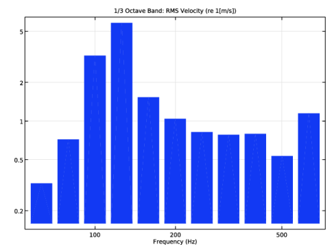
In the Settings window for 1D Plot Group, type Velocity, X-component RMS 1/3 Octave in the Label text field.
3
Locate the Title section. From the Title type list, choose Manual.
4
In the Title text area, type 1/3 Octave Band: RMS Velocity (re 1[m/s]).
5
Locate the Axis section. Select the x-axis log scale checkbox.
6
Select the y-axis log scale checkbox.
7
Click the  Show More Options button in the Model Builder toolbar.
8
In the Show More Options dialog, in the tree, select the checkbox for the node Results > All Plot Types.
9
Octave Band 1
1
In the Velocity, X-component RMS 1/3 Octave toolbar, click  More Plots and choose Octave Band.
2
3
In the Settings window for Octave Band, locate the y-Axis Data section.
4
In the Expression text field, type abs(solid.u_tX)/sqrt(2).
5
From the Expression type list, choose General (non-dB).
6
In the Reference expression text field, type 1[m/s].
7
Locate the Plot section. From the Band type list, choose 1/3 octave.
8
In the Velocity, X-component RMS 1/3 Octave toolbar, click  Plot.
You will now consider a static load applied to the bracket and perform a prestressed frequency domain analysis.
Add Study
1
In the Home toolbar, click  Add Study to open the Add Study window.
2
Go to the Add Study window.
3
Find the Studies subsection. In the Select Study tree, select Preset Studies for Selected Physics Interfaces > Frequency Domain, Prestressed.
4
Click the Add Study button in the window toolbar.
5
In the Home toolbar, click  Add Study to close the Add Study window.
Global Definitions
Parameters 1
1
In the Settings window for Parameters, locate the Parameters section.
2
Solid Mechanics (solid)
Boundary Load, Prestress
1
In the Physics toolbar, click  Boundaries and choose Boundary Load.
Apply a boundary load to the bracket holes.
2
In the Settings window for Boundary Load, type Boundary Load, Prestress in the Label text field.
3
Locate the Boundary Selection section. From the Selection list, choose Pin Holes.
4
Locate the Coordinate System Selection section. From the Coordinate system list, choose Boundary System 1 (sys1).
5
Locate the Force section. Specify the fA vector as
The default boundary system is in the deformed configuration. This would make the load behave as a follower load when used in a geometrically nonlinear context. Change to a fixed coordinate system.
Definitions
Boundary System 1 (sys1)
1
In the Model Builder window, expand the Component 1 (comp1) > Definitions node, then click Boundary System 1 (sys1).
2
In the Settings window for Boundary System, locate the Settings section.
3
From the Frame list, choose Reference configuration.
Study 2
Step 2: Frequency-Domain Perturbation
1
In the Model Builder window, under Study 2 click Step 2: Frequency-Domain Perturbation.
2
In the Settings window for Frequency-Domain Perturbation, locate the Study Settings section.
3
In the Frequencies text field, type range(50,10,90) range(91,1,149) range(150,10,200).
4
In the Study toolbar, click  Compute.
Results
1
Click the  Zoom Extents button in the Graphics toolbar.
You have previously created a point graph plot for the unloaded case. Add a new point graph plot to the same figure but use the dataset of the second load case.
Point Graph 1, Point Graph 2
1
In the Model Builder window, under Results > Displacement, RMS, Ctrl-click to select Point Graph 1 and Point Graph 2.
2
Point Graph 3
1
In the Settings window for Point Graph, locate the Data section.
2
From the Dataset list, choose Study 2/Solution 3 (sol3).
3
Locate the Coloring and Style section. From the Color list, choose Cycle (reset).
4
Find the Line style subsection. From the Line list, choose Dashed.
5
Find the Line markers subsection. From the Marker list, choose None.
6
Locate the Legends section. In the table, enter the following settings:
Estimate the damping from the response using the full width at half maximum (FWHM) method. Since this method is based on a power definition, the corresponding level for an amplitude variable is the peak value divided by 2. Note that a table containing the damping values is automatically generated.
Graph Marker 1
1
In the Model Builder window, expand the Point Graph 3 node, then click Graph Marker 1.
2
In the Settings window for Graph Marker, locate the Display section.
3
From the Display mode list, choose Bandwidth.
4
From the Cutoff mode list, choose Relative to peak.
5
Locate the Coloring and Style section. From the Color list, choose Blue.
6
In the Displacement, RMS toolbar, click  Plot.
Point Graph 4
1
In the Model Builder window, under Results > Displacement, RMS click Point Graph 4.
2
In the Settings window for Point Graph, locate the Data section.
3
From the Dataset list, choose Study 2/Solution 3 (sol3).
4
Locate the Coloring and Style section. Find the Line style subsection. From the Line list, choose Dashed.
5
Locate the Legends section. In the table, enter the following settings:
6
In the Displacement, RMS toolbar, click  Plot.
Displacement, RMS
1
In the Model Builder window, click Displacement, RMS.
2
In the Settings window for 1D Plot Group, locate the Axis section.
3
Select the Manual axis limits checkbox.
4
In the x minimum text field, type 49.
5
In the x maximum text field, type 220.
6
In the y minimum text field, type 0.02.
7
In the y maximum text field, type 1.1.
8
Locate the Legend section. From the Position list, choose Upper left.
9
In the Displacement, RMS toolbar, click  Plot.
Volume 1
1
In the Model Builder window, expand the Stress (solid) 1 node, then click Volume 1.
2
In the Settings window for Volume, locate the Expression section.
3
In the Expression text field, type solid.misesGp.
4
Locate the Coloring and Style section. From the Color table list, choose Rainbow.
What is shown here is the deviation from the prestress value. This is why the von Mises stress can be negative.
Stress (solid), Prestressed
1
In the Model Builder window, expand the Results > Datasets node, then click Results > Stress (solid) 1.
2
In the Settings window for 3D Plot Group, type Stress (solid), Prestressed in the Label text field.
Exactly at a resonance, there will be a phase shift of 90 degrees between load and displacement. In order to see the highest stresses, it is necessary to plot the results at another phase angle.
3
Locate the Phase section. From the Solution at angle (phase) list, choose Manual.
4
In the Phase text field, type 90.
Investigate the stress distribution around the resonances.
5
Locate the Data section. From the Parameter value (freq (Hz)) list, choose 105.
6
Click the  Transparency button in the Graphics toolbar.
7
Click the  Show Grid button in the Graphics toolbar.
8
Click the  Zoom Extents button in the Graphics toolbar.
9
From the Parameter value (freq (Hz)) list, choose 128.
10
In the Stress (solid), Prestressed toolbar, click  Plot.
Now plot the phase shift with respect to the applied load phase.
Displacement Phase, X Component
1
In the Model Builder window, right-click Displacement, RMS and choose Duplicate.
2
In the Model Builder window, click Displacement, RMS 1.
3
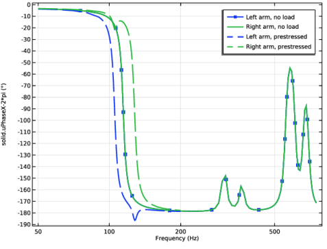
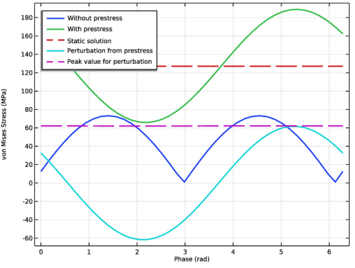
In the Settings window for 1D Plot Group, type Displacement Phase, X Component in the Label text field.
4
Click the  y-Axis Log Scale button in the Graphics toolbar.
5
Locate the Axis section. Clear the Manual axis limits checkbox.
6
Locate the Legend section. From the Position list, choose Upper right.
Point Graph 1
1
In the Model Builder window, click Point Graph 1.
2
In the Settings window for Point Graph, locate the y-Axis Data section.
3
In the Expression text field, type solid.uPhaseX-2*pi.
4
From the Unit list, choose °.
Graph Marker 1
1
In the Model Builder window, expand the Point Graph 1 node.
2
Right-click Graph Marker 1 and choose Delete.
Point Graph 2
1
In the Model Builder window, under Results > Displacement Phase, X Component click Point Graph 2.
2
In the Settings window for Point Graph, locate the y-Axis Data section.
3
In the Expression text field, type solid.uPhaseX-2*pi.
4
From the Unit list, choose °.
Point Graph 3
1
In the Model Builder window, click Point Graph 3.
2
In the Settings window for Point Graph, locate the y-Axis Data section.
3
In the Expression text field, type solid.uPhaseX-2*pi.
4
From the Unit list, choose °.
Graph Marker 1
1
In the Model Builder window, expand the Point Graph 3 node.
2
Right-click Graph Marker 1 and choose Delete.
Point Graph 4
1
In the Model Builder window, under Results > Displacement Phase, X Component click Point Graph 4.
2
In the Settings window for Point Graph, locate the y-Axis Data section.
3
In the Expression text field, type solid.uPhaseX-2*pi.
4
From the Unit list, choose °.
Add a plot showing the time history of the displacement over a period for two points and two frequencies.
Displacement History
1
In the Results toolbar, click  1D Plot Group.
2
In the Settings window for 1D Plot Group, type Displacement History in the Label text field.
3
Locate the Data section. From the Dataset list, choose Study 2/Solution 3 (sol3).
4
From the Parameter selection (freq) list, choose From list.
5
In the Parameter values (freq (Hz)) list, select 105.
6
Locate the Title section. From the Title type list, choose None.
Point Graph 1
1
Right-click Displacement History and choose Point Graph.
2
3
In the Settings window for Point Graph, locate the y-Axis Data section.
4
In the Expression text field, type u.
5
Locate the x-Axis Data section. From the Parameter list, choose Phase.
6
Locate the Coloring and Style section. From the Width list, choose 2.
7
In the Displacement History toolbar, click  Plot.
8
Locate the Legends section. Select the Show legends checkbox.
9
From the Legends list, choose Manual.
10
Point Graph 2
1
Right-click Point Graph 1 and choose Duplicate.
2
In the Settings window for Point Graph, locate the Selection section.
3
Click  Clear Selection.
4
5
Locate the Legends section. In the table, enter the following settings:
6
In the Displacement History toolbar, click  Plot.
Point Graph 1, Point Graph 2
1
In the Model Builder window, under Results > Displacement History, Ctrl-click to select Point Graph 1 and Point Graph 2.
2
Point Graph 3
1
In the Settings window for Point Graph, locate the Data section.
2
From the Dataset list, choose Study 2/Solution 3 (sol3).
3
From the Parameter selection (freq) list, choose From list.
4
In the Parameter values (freq (Hz)) list, select 128.
5
Locate the Coloring and Style section. Find the Line style subsection. From the Line list, choose Dashed.
6
From the Color list, choose Cycle (reset).
7
Locate the Legends section. In the table, enter the following settings:
8
In the Displacement History toolbar, click  Plot.
Point Graph 4
1
In the Model Builder window, click Point Graph 4.
2
In the Settings window for Point Graph, locate the Data section.
3
From the Dataset list, choose Study 2/Solution 3 (sol3).
4
From the Parameter selection (freq) list, choose From list.
5
In the Parameter values (freq (Hz)) list, select 128.
6
Locate the Coloring and Style section. Find the Line style subsection. From the Line list, choose Dashed.
7
Locate the Legends section. In the table, enter the following settings:
8
In the Displacement History toolbar, click  Plot.
Add a plot showing the time history of the von Mises stress at resonance over a period for a certain point.
von Mises History
1
In the Results toolbar, click  1D Plot Group.
2
In the Settings window for 1D Plot Group, locate the Data section.
3
From the Parameter selection (freq) list, choose From list.
4
In the Parameter values (freq (Hz)) list, select 114.
5
Locate the Title section. From the Title type list, choose None.
6
In the Label text field, type von Mises History.
Point Graph 1
1
Right-click von Mises History and choose Point Graph.
2
3
In the Settings window for Point Graph, locate the y-Axis Data section.
4
In the Expression text field, type solid.mises.
5
Locate the x-Axis Data section. From the Parameter list, choose Phase.
6
In the Phase text field, type (pi/20)*range(0,1,40).
7
Locate the Legends section. Select the Show legends checkbox.
8
From the Legends list, choose Manual.
9
10
In the von Mises History toolbar, click  Plot.
Point Graph 2
1
Right-click Point Graph 1 and choose Duplicate.
2
In the Settings window for Point Graph, locate the Data section.
3
From the Dataset list, choose Study 2/Solution 3 (sol3).
4
From the Parameter selection (freq) list, choose From list.
5
In the Parameter values (freq (Hz)) list, select 107.
6
Locate the Legends section. In the table, enter the following settings:
7
Locate the y-Axis Data section. From the Expression evaluated for list, choose Total instantaneous solution.
8
In the von Mises History toolbar, click  Plot.
Point Graph 3
1
Right-click Point Graph 2 and choose Duplicate.
2
In the Settings window for Point Graph, locate the y-Axis Data section.
3
From the Expression evaluated for list, choose Static solution.
4
Locate the Legends section. In the table, enter the following settings:
5
In the von Mises History toolbar, click  Plot.
Point Graph 4
1
Right-click Point Graph 3 and choose Duplicate.
2
In the Settings window for Point Graph, locate the y-Axis Data section.
3
From the Expression evaluated for list, choose Harmonic perturbation.
4
Select the Compute differential checkbox.
5
Locate the Legends section. In the table, enter the following settings:
6
In the von Mises History toolbar, click  Plot.
Point Graph 5
1
Right-click Point Graph 4 and choose Duplicate.
2
In the Settings window for Point Graph, locate the y-Axis Data section.
3
In the Expression text field, type solid.mises_peak.
4
Locate the Legends section. In the table, enter the following settings:
5
Locate the y-Axis Data section. Clear the Compute differential checkbox.
6
Locate the Coloring and Style section. Find the Line style subsection. From the Line list, choose Dashed.
7
In the von Mises History toolbar, click  Plot.
Point Graph 3
1
In the Model Builder window, click Point Graph 3.
2
In the Settings window for Point Graph, locate the Coloring and Style section.
3
Find the Line style subsection. From the Line list, choose Dashed.
von Mises History
1
In the Model Builder window, click von Mises History.
2
In the Settings window for 1D Plot Group, locate the Plot Settings section.
3
Select the y-axis label checkbox. In the associated text field, type von Mises Stress (MPa).
4
Locate the Legend section. From the Position list, choose Upper left.
5
In the von Mises History toolbar, click  Plot.