|
|
|
|
1
|
|
2
|
|
3
|
Click Add.
|
|
4
|
Click
|
|
5
|
|
6
|
Click
|
|
1
|
|
2
|
|
3
|
|
1
|
|
2
|
|
3
|
Click
|
|
4
|
Browse to the model’s Application Libraries folder and double-click the file superlattice_band_gap_tool.txt.
|
|
1
|
|
2
|
|
3
|
|
4
|
|
6
|
Click
|
|
1
|
|
2
|
In the Settings window for Schrödinger Equation, type Schrödinger Equation e- in the Label text field.
|
|
3
|
|
4
|
Click to expand the Dependent Variables section. In the Wave functions (1) table, enter the following settings:
|
|
1
|
In the Model Builder window, under Component 1 (comp1) > Schrödinger Equation e- (schre) click Effective Mass 1.
|
|
2
|
|
3
|
|
1
|
|
2
|
|
3
|
|
1
|
|
3
|
|
4
|
|
1
|
|
3
|
|
4
|
|
1
|
|
2
|
|
3
|
|
1
|
|
2
|
Go to the Add Physics window.
|
|
3
|
|
4
|
Click the Add to Component 1 button in the window toolbar.
|
|
5
|
|
1
|
In the Settings window for Schrödinger Equation, type Schrödinger Equation hole in the Label text field.
|
|
2
|
|
3
|
|
4
|
Locate the Dependent Variables section. In the Wave functions (1) table, enter the following settings:
|
|
1
|
In the Model Builder window, under Component 1 (comp1) > Schrödinger Equation hole (schrh) click Effective Mass 1.
|
|
2
|
|
3
|
|
1
|
|
2
|
|
3
|
|
1
|
|
3
|
|
4
|
|
1
|
|
3
|
|
4
|
|
1
|
|
2
|
|
3
|
|
1
|
|
2
|
|
3
|
Click the Custom button.
|
|
4
|
|
5
|
Click
|
|
1
|
|
2
|
|
3
|
|
4
|
|
5
|
Locate the Physics and Variables Selection section. In the Solve for column of the table, under Component 1 (comp1), clear the checkbox for Schrödinger Equation hole (schrh).
|
|
6
|
|
7
|
|
8
|
Clear the Generate default plots checkbox.
|
|
9
|
|
1
|
|
2
|
Go to the Add Study window.
|
|
3
|
Find the Studies subsection. In the Select Study tree, select Preset Studies for Selected Physics Interfaces > Eigenvalue.
|
|
4
|
Find the Physics interfaces in study subsection. In the table, clear the Solve checkbox for Schrödinger Equation e- (schre).
|
|
5
|
Click the Add Study button in the window toolbar.
|
|
6
|
|
1
|
|
2
|
|
3
|
|
4
|
|
5
|
|
6
|
Clear the Generate default plots checkbox.
|
|
7
|
|
1
|
|
2
|
|
3
|
|
4
|
|
5
|
|
6
|
|
7
|
|
8
|
|
1
|
|
2
|
|
3
|
|
4
|
|
5
|
|
1
|
|
2
|
|
3
|
|
4
|
Locate the Expressions section. In the table, enter the following settings:
|
|
5
|
Click
|
|
1
|
|
2
|
|
3
|
|
4
|
Locate the Expressions section. In the table, enter the following settings:
|
|
5
|
Click
|
|
1
|
|
2
|
|
3
|
|
4
|
Locate the Expressions section. In the table, enter the following settings:
|
|
5
|
Click
|
|
1
|
|
2
|
|
3
|
|
4
|
|
5
|
Locate the Plot Settings section.
|
|
6
|
|
7
|
|
8
|
|
1
|
|
2
|
|
3
|
|
4
|
|
5
|
|
6
|
|
7
|
|
8
|
|
9
|
|
10
|
|
11
|
|
12
|
|
1
|
|
2
|
|
3
|
|
4
|
|
5
|
|
6
|
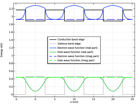
Locate the Legends section. In the table, enter the following settings:
|
|
1
|
|
2
|
|
3
|
Locate the y-Axis Data section. In the Expression text field, type data1(schre.Psi*Egw/4/schre.plot_fac+schre.Ei/e_const).
|
|
4
|
|
5
|
|
6
|
Locate the Legends section. In the table, enter the following settings:
|
|
1
|
|
2
|
|
3
|
Locate the y-Axis Data section. In the Expression text field, type data2(-schrh.Psi*Egw/4/schrh.plot_fac-schrh.Ei/e_const).
|
|
4
|
|
5
|
Locate the Legends section. In the table, enter the following settings:
|
|
1
|
|
2
|
|
3
|
Locate the y-Axis Data section. In the Expression text field, type data1(imag(schre.Psi)*Egw/4/schre.plot_fac+schre.Ei/e_const).
|
|
4
|
Locate the Coloring and Style section. Find the Line style subsection. From the Line list, choose Dashed.
|
|
5
|
|
6
|
Locate the Legends section. In the table, enter the following settings:
|
|
1
|
|
2
|
|
3
|
Locate the y-Axis Data section. In the Expression text field, type data2(-imag(schrh.Psi)*Egw/4/schrh.plot_fac-schrh.Ei/e_const).
|
|
4
|
Locate the Coloring and Style section. Find the Line style subsection. From the Line list, choose Dashed.
|
|
5
|
|
6
|
Locate the Legends section. In the table, enter the following settings:
|
|
7
|