COMSOL 6.3 - Diffraction Grating

This tutorial uses the Wave Optics Module and the Ray Optics Module to simulate the propagation of rays through a diffraction grating at different angles of incidence. It uses the S-parameters computed by the Electromagnetic Waves, Frequency Domain interface on a unit cell of the grating to specify the reflectance and transmittance of each diffraction order in the Geometrical Optics interface, allowing ray propagation through the grating to be modeled over length scales much larger than the width of the unit cell.

The Geometrical Optics interface includes a feature that can be used to simulate propagation of electromagnetic waves on fully scaled optical devices without the need to spatially resolve the wavelength, which would be impractical in many cases due to the large number of mesh elements required.

Although the directions of propagation for the diffraction orders can be derived from the wavelength of radiation, the angle of incidence, and the width of a unit cell in the grating, reinitialization of the ray intensity requires prior calculation of the transmittance and reflectance for all diffraction orders as a function of angle of incidence. These quantities can be obtained by computing the S-parameters of each diffraction order for a single unit cell as a function of the angle of incidence using the and features for the Electromagnetic Waves, Frequency Domain interface.

This 2D model is separated in two parts.

•

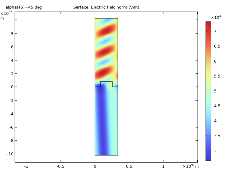
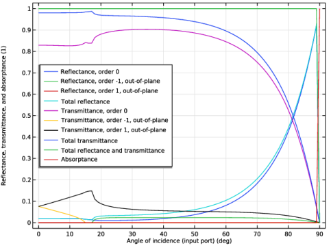
First, the transmittance and reflectance of each diffraction order are computed using the Electromagnetic Waves, Frequency Domain interface on a single unit cell of the grating. For this part of the model it is necessary to fully resolve the wavelength. A is used to compute the transmittance and reflectance as functions of the angle of incidence.

•

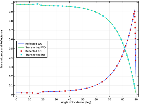
The second part demonstrates how the transmittance and reflectance values can be used to generate a set of interpolation functions that can be used with the feature of the Geometrical Optics interface.

Model Definition

This model simulates the interaction of light of free-space wavelength λ0 = 441 nm with a 5 mm wide dielectric grating of grating constant (the distance between the grooves) d = 340 nm.

Notes on Diffraction orders

For a plane wave incident on a diffraction grating at angle of incidence α (SI unit: rad) as in Figure 1, the diffraction orders correspond to the angles at which the difference in optical path length for wavefronts from adjacent unit cells is an integer multiple of the wavelength. The angle of a transmitted order βm (SI unit: rad) is defined by the relation

where the diffraction order m (dimensionless) is an integer.

Figure 1: The geometric path lengths of two transmitted parallel rays.The shaded area represents a unit cell of the diffraction grating (SiO2). For this model the grating constant is d = 340 nm and the monochromatic TE polarized light has a wavelength of λ0 = 441 nm.

For m = 0, the angle of refraction is described by Snell’s law,

For reflected rays, nα = nβ. For m = 0, specular reflection occurs, β0 = α.

Because the sine functions can only vary between −1 and 1, the existence of higher diffraction orders requires that

In this example only the diffraction orders 0, 1, and −1 can be released, which means that

As mentioned in the introduction, the model consists of two parts: the S-parameter calculation using a single unit cell and the ray trajectory computation in an optically large modeling domain.

S-parameter Calculation

The transmittance and reflectance for the refraction, specular reflection, and first order diffraction of plane TE waves (electric field component in the z direction, out of the xy-plane) are computed for a single unit cell.

The Electromagnetic Waves, Frequency Domain interface is used to model wave propagation in a single unit cell of the grating, as outlined in Figure 1. On either side of the unit cell, the boundary condition with is used. This condition states that the solution on one side of the unit cell equals the solution on the other side multiplied by a complex-valued phase factor. The phase shift between the boundaries is evaluated from the perpendicular component of the wave vector. Note that due to the continuity of the field, the phase factor is the same for the refracted and reflected waves as for the incident wave.

boundary conditions are used to release the incident wave and to absorb the reflected and transmitted waves of order 0. To ensure that no unphysical reflections occur, subnodes must be added to the nodes to absorb outgoing waves of each nonzero diffraction order.

The input to each periodic port is an electric field amplitude vector and an angle of incidence. In this example the angle of incidence is swept from 0° to 90° at 1° intervals.

Ray Tracing

The Geometrical Optics interface computes the intensity of rays of each diffraction order using the transmittance and reflectance computed in the previous study. In order to see the effect of the angle of incidence on the ray trajectories and intensity, 901 rays are released from a point in a 90° cone with a source power density of 901 W/m, or 1 W/m per ray. For each diffraction order, two rays may be released, one transmitted ray and one reflected ray. Because the transmitted ray of order 0 uses the same degrees of freedom as the incident ray, five extra degrees of freedom should be allocated per incident ray: one for the reflected ray of order 0 and two each for the reflected and transmitted rays of order m = 1 and m = −1. A total of 4505 secondary rays are allocated.

Use of Sign Conventions for Diffraction Orders

The Electromagnetic Waves physics interfaces use a different sign convention to distinguish between positive and negative diffraction orders, compared to the Geometrical Optics interfaces.

In the Electromagnetic Waves interface in this model, the excited port is at the top of the geometry and the waves propagate downward. Increases in diffraction order correspond to clockwise rotations of both the reflected and transmitted wave vectors on either side of the unit cell. Thus higher reflected orders point more to the right, while higher transmitted orders point more to the left.

In contrast, the Geometrical Optics interface increments the tangential component of the wave vector by the same multiple of the reciprocal lattice vector for both transmitted and reflected rays of each diffraction order. Higher diffraction orders point more to the right for both reflected and transmitted rays.

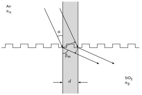
Therefore, when using the solution of the Electromagnetic Waves interface to reinitialize the power of rays, pay careful attention to how the diffraction orders are negated for transmitted rays:

•

For the node, the specified and are R0(alpha_ro) and T0(alpha_ro), respectively. Here alpha_ro is a variable for the angle of incidence of each ray, measured counterclockwise from the surface normal.

•

For the node, the specified is Rm1(alpha_ro) and the specified is T1(alpha_ro). The m = −1 order for reflected rays corresponds to the m = −1 order for reflected waves, but the m = −1 order for transmitted rays corresponds to the m = +1 order for transmitted waves.

•

For the node, the specified is R1(alpha_ro) and the specified is T1(alpha_ro). The m = +1 order for reflected rays corresponds to the m = +1 order for reflected waves, but the m = +1 order for transmitted rays corresponds to the m = −1 order for transmitted waves.

This tutorial would require further extension if rays could also be released from the upper-right quadrant, propagating downward and to the left. As currently defined, alpha_ro is negative for rays propagating downward and to the left. The interpolation functions used to specify the reflectance and transmittance for rays of each diffraction order are only defined for positive angles.

Results and Discussion

The electric field norm for a TE wave with an angle of incidence of 45° is shown in Figure 2. In order to get reliable results one has to use a very fine mesh to resolve the wavelength. To resolve a wave properly, it is necessary to use about 10 mesh elements per wavelength when using linear shape functions, or 5 elements per wavelength when using the default quadratic shape functions.

Figure 2: Norm of the electric field for a TE wave with an angle of incidence of 45 degrees.

The transmittance and reflectance of each diffraction order as functions of the angle of incidence are shown in Figure 3. Most of the radiation is transmitted at diffraction order 0, except at very large angles of incidence for which most of the radiation is reflected.

Figure 3: Reflectance and transmittance of diffraction orders 0, 1, and -1 as functions of the angle of incidence.

The raw data from Figure 3 was used to define a series of six interpolation functions, each corresponding to the reflectance or transmittance of a diffraction order. These interpolation functions were used in the Geometrical Optics interface to define the reinitialized intensity of the transmitted and reflected rays.

In Figure 4 the total intensity of the reflected and transmitted rays, indicated by points at discrete angle intervals, is compared to the sum of the reflectance and transmittance functions defined with the solution data from full wave solution.

The curves for the Electromagnetic Waves, Frequency Domain interface and the Geometrical Optics interface agree closely, which is to be expected because the transmittance and reflectance of the grating in the latter are defined explicitly in terms of the solution to the former.

Figure 4: The transmittance and reflectance computed by both the wave optics and ray optics models.

Ray_Optics_Module/Verification_Examples/diffraction_grating

Modeling Instructions

From the menu, choose .

New

In the window, click

Model Wizard

In the window, click

In the tree, select > > .

Click .

Click

In the tree, select > .

Click

Global Definitions

Parameters 1

In the window, under click .

In the window for , locate the section.

In the table, enter the following settings:


Name	Expression	Value	Description
n_air	1	1	Refractive index air
n_sio2	1.54874	1.5487	Refractive index SiO2
d	340[nm]	3.4E-7 m	Grating constant
lam0	441[nm]	4.41E-7 m	Vacuum wavelength of incident light
f0	c_const/lam0	6.798E14 1/s	Frequency of incident light
alpha	0.0[deg]	0 rad	Angle of incidence (input port)

Because this model uses two model Components with different geometries but the same material properties, it is convenient to define global materials before setting up the individual physics interfaces.

Air

In the window, under right-click and choose .

In the window for , type Air in the text field.

Click to expand the section. In the tree, select > > .

Click

Locate the section. In the table, enter the following settings:


Property	Variable	Value	Unit	Property group
Refractive index, real part	n_iso ; nii = n_iso, nij = 0	n_air	1	Refractive index
Refractive index, imaginary part	ki_iso ; kiii = ki_iso, kiij = 0	0	1	Refractive index

SiO2

Right-click and choose .

In the window for , type SiO2 in the text field.

Click to expand the section. In the tree, select > > .

Click

Locate the section. In the table, enter the following settings:


Property	Variable	Value	Unit	Property group
Refractive index, real part	n_iso ; nii = n_iso, nij = 0	n_sio2	1	Refractive index
Refractive index, imaginary part	ki_iso ; kiii = ki_iso, kiij = 0	0	1	Refractive index

Geometry 1

Create the geometry of a single unit cell in the grating.

Rectangle 1 (r1)

In the toolbar, click

In the window for , locate the section.

In the text field, type d.

In the text field, type 6*d.

Locate the section. In the text field, type -3*d.

Rectangle 2 (r2)

In the toolbar, click

In the window for , locate the section.

In the text field, type d.

In the text field, type 3*d.

Locate the section. In the text field, type -3*d.

Rectangle 3 (r3)

In the toolbar, click

In the window for , locate the section.

In the text field, type d/2.

In the text field, type d/4.

Locate the section. In the text field, type d/4.

Union 1 (uni1)

In the toolbar, click

and choose .

Select the objects and only.

In the window for , locate the section.

Clear the checkbox.

Click

. The geometry should look like the unit cell in Figure 1.

Materials

Material Link 1 (matlnk1)

In the window, under right-click and choose > .

Select Domain 2 only.

Material Link 2 (matlnk2)

Right-click and choose > .

Select Domain 1 only.

In the window for , locate the section.

From the list, choose .

Study 1

Step 1: Frequency Domain

It is convenient to specify the frequency in the sweep before setting up the physics, since it can then be used to automatically compute the diffraction orders for the boundary conditions.

In the window, under click .

In the window for , locate the section.

In the text field, type f0.

In this model the S-parameters of a TE wave are computed. Select as the component of the electric field to be solved for.

Electromagnetic Waves, Frequency Domain (ewfd)

In the window, under click .

In the window for , locate the section.

From the list, choose .

Create a periodic input port. To model a TE wave, keep the as the .

Port 1

In the toolbar, click

and choose .

Select Boundary 5 only.

In the window for , locate the section.

From the list, choose .

Locate the section. In the α text field, type alpha.

Locate the section. From the list, choose , to add nodes that are propagating for non-normal incidence.

Add the output port. In this case the excitation is set to .

Port 2

In the toolbar, click

and choose .

Select Boundary 2 only.

In the window for , locate the section.

From the list, choose .

Add the nodes for the second periodic port by clicking the button on the first periodic port.

Port 1

In the window, click .

In the window for , locate the section.

Click .

Add the periodic boundary condition to the sides of the unit cell.

Periodic Condition 1

In the toolbar, click

and choose .

Select Boundaries 1, 3, 10, and 11 only.

In the window for , locate the section.

From the list, choose .

Study 1

Parametric Sweep

In the toolbar, click

In the window for , locate the section.

Click

In the table, enter the following settings:


Parameter name	Parameter value list	Parameter unit
alpha (Angle of incidence (input port))	range(0,1,90)	deg

In the toolbar, click

Results

Electric Field (ewfd)

In the window for , locate the section.

From the list, choose .

In the toolbar, click

Click the

button in the toolbar. Compare the resulting plot to Figure 2.

Global Evaluation 1

In the toolbar, click

In the window for , locate the section.

In the table, enter the following settings:


Expression	Unit	Description
ewfd.Rorder_0	1	R0
ewfd.Torder_0	1	T0
ewfd.Rorder_n1_op	1	R-1
ewfd.Torder_n1_op	1	T-1
ewfd.Rorder_p1_op	1	R1
ewfd.Torder_p1_op	1	T1

Click

. The resulting table shows the reflectance and transmittance values as functions of the angle of incidence.

Reflectance, Transmittance, and Absorptance (ewfd)

A line plot for the reflectances, transmittances, and absorptance is also generated by default. Move the legend panel to not cover the line plots.

In the window, under click .

In the window for , locate the section.

From the list, choose . Compare the resulting plot to Figure 3.

Now add a second model Component to compute the ray trajectories.

Add Component

In the window, right-click the root node and choose > .

Geometry 2

Rectangle 1 (r1)

In the toolbar, click

In the window for , locate the section.

From the list, choose .

Locate the section. In the text field, type 5[mm].

In the text field, type 1.35[mm].

Rectangle 2 (r2)

In the toolbar, click

In the window for , locate the section.

In the text field, type 5[mm].

Locate the section. From the list, choose .

Locate the section. In the text field, type 0.675[mm].

Locate the section. In the text field, type -0.675[mm]/2.

Click

Definitions (comp2)

Use the reflectance and transmittance data from the previous study to define a series of interpolation functions for the large-scale geometrical optics analysis.

Interpolation 1 (int1)

In the toolbar, click

In the window for , locate the section.

From the list, choose .

Locate the section. In the table, enter the following settings:


Columns	Type	Settings
R0 (1)	Function values	Function name=int1
T0 (1)	Function values	Function name=int1a
R-1 (1)	Function values	Function name=int1b
T-1 (1)	Function values	Function name=int1c
R1 (1)	Function values	Function name=int1d
T1 (1)	Function values	Function name=int1e

In the table, click to select the cell at row number 1 and column number 1.

In the text field, type deg.

In the table, click to select the cell at row number 2 and column number 1.

In the text field, type R0.

In the text field, type 1.

In the table, click to select the cell at row number 3 and column number 1.

In the text field, type T0.

In the text field, type 1.

In the table, click to select the cell at row number 4 and column number 1.

In the text field, type Rm1.

In the text field, type 1.

In the table, click to select the cell at row number 5 and column number 1.

In the text field, type Tm1.

In the text field, type 1.

In the table, click to select the cell at row number 6 and column number 1.

In the text field, type R1.

In the text field, type 1.

In the table, click to select the cell at row number 7 and column number 1.

In the text field, type T1.

In the text field, type 1.

Now set up the Geometrical Optics interface.

Add Physics

In the toolbar, click

to open the window.

Go to the window.

In the tree, select > > .

Click the button in the window toolbar.

In the toolbar, click

to close the window.

Materials

Material Link 3 (matlnk3)

In the window, under right-click and choose > .

Select Domain 2 only.

Material Link 4 (matlnk4)

Right-click and choose > .

Select Domain 1 only.

In the window for , locate the section.

From the list, choose .

Geometrical Optics (gop)

In the window, under click .

In the window for , locate the section.

From the list, choose .

Locate the section. In the text field, type 4505.

Ray Properties 1

In the window, under > click .

In the window for , locate the section.

From the list, choose .

In the ν text field, type f0.

Define the angle of incidence as a function of the wave vector.

Definitions (comp2)

Variables 1

In the window, under right-click and choose .

In the window for , locate the section.

In the table, enter the following settings:


Name	Expression	Unit	Description
alpha_ro	atan2(kx,-ky)	rad

Geometrical Optics (gop)

Grating 1

In the toolbar, click

and choose .

Select Boundary 4 only.

In the window for , locate the section.

In the d text field, type d.

Select the checkbox.

These checkboxes create variables that can be used to compute the total power of all transmitted rays and all reflected rays, respectively, for each angle of incidence.

By default a subnode is created to release rays of order 0. Modify this default subnode, then create additional subnodes to release rays of diffraction orders +1 and -1.

Diffraction Order (m = 0)

In the window, expand the node, then click .

In the window for , locate the section.

In the R text field, type R0(alpha_ro).

In the T text field, type T0(alpha_ro).

Grating 1

In the window, click .

Diffraction Order (m = 1)

In the toolbar, click

and choose .

In the window for , locate the section.

In the m text field, type -1.

In the R text field, type Rm1(alpha_ro).

In the T text field, type T1(alpha_ro).

Grating 1

In the window, click .

Diffraction Order (m = 1)

In the toolbar, click

and choose .

In the window for , locate the section.

In the R text field, type R1(alpha_ro).

In the T text field, type Tm1(alpha_ro).

Release from Grid 1

In the toolbar, click

and choose .

In the window for , locate the section.

In the qy,0 text field, type 1e-6. The ray will be released an extremely short distance above the grating so that even rays at very large angles of incidence will reach the boundary fairly quickly.

Locate the section. From the list, choose .

In the Nw text field, type 901.

In the α text field, type pi/4.

Specify the r vector as