PDF

Resin Transfer Molding of a Wind Turbine Blade
Introduction
Resin Transfer Molding (RTM) is a manufacturing process for composite structures. The resin is injected under pressure into the mold cavity. Reinforcement materials like fiber structures can be placed into the empty mold before the resin is injected, which makes it easier to use any kind of reinforcement material and orientation. After the resin has been injected the curing takes place.
To avoid air bubbles that might be trapped within the resin several vents are placed at certain positions of the mold. Simulation can be used to optimize the vent positions.
In this example the RTM process of a wind turbine blade is investigated. The model geometry and setup was inspired by Ref. 1.
Model Definition
The blade consists of five parts of different composites, which have different anisotropic permeabilities. The colors in Figure 1 indicate the different permeabilities. The blade has a thickness of 1 cm. The geometry was constructed using COMSOL Multiphysics and the Design Module. However, in this example we just import the ready-made geometry file.
Figure 1: Geometry of the wind turbine blade. The colors indicate the different porous materials and different permeabilities.
Initially, the blade is filled with air. Resin is injected via the cylindrical inlet pipes at the top of the blade with a pressure of 800 kPa. The air can escape through the outlets which are defined at both short ends of the blade and at four additional vents along the blade rim which are marked by the outgoing arrows in Figure 1. All other boundaries are assumed as solid walls and the No Slip wall condition applies.
The model is set up using the combined multiphysics interface Two Phase Flow, Level Set, Brinkman Equations.
Model Equations
The flow through the porous media within the mold (due to the reinforcement material) is described by the Brinkman Equations for incompressible flow:
(1)
In these equations, where the inertial term has been neglected, μ (SI unit: kg/(m·s)) is the dynamic viscosity of the fluid, u (SI unit: m/s) is the velocity vector, ρ (SI unit: kg/m3) is the density of the fluid, p (SI unit: Pa) is the pressure, εp is the porosity, and κ (SI unit: m2) the permeability of the porous medium.
For the two-phase flow level-set method, an equation for the level-set function ϕ, which describes the interface between the two phases, is solved:
(2)
In this equation, ϕ is a smoothed step function which is zero within one phase and one within the other, ε denotes the porosity, γ determines the amount of reinitialization, and εls describes the thickness of the interface.
Beside defining the interface between the two phases, the level-set function is used in the multiphysics coupling feature node Two-Phase Flow, Level Set to smoothen the density and viscosity jumps across the interface through the definitions
(3)
Table 1 lists the parameters that are used in the model.
10-5 Pa·s
2.9·10-10, 8·10-11, 2.9·10-10 m2
2.5·10-10, 7·10-11, 2.5·10-10 m2
1.7·10-10, 8·10-11, 1.7·10-10 m2
Results and Discussion
Figure 2: Velocity magnitude in logarithmic scale (color plot) and tangential velocity (arrow plot) along the mold surface.
After about 45 minutes of simulated time, the mold is filled to 95% with resin. Figure 2 shows the velocity magnitude along the mold surface. The highest velocity values appear near the inlets and the small vents, where the flow channel narrows.
Figure 3 shows the pressure at the external surfaces of the blade. The highest pressure appears at the inlets.
Figure 3: Pressure plotted on the external surfaces of the wind turbine blade.
Figure 4: Volume fraction of resin after 15 minutes of simulated time.
The resin front advances as shown in Figure 4 and Figure 5. In Figure 4, the resin front is shown after 15 minutes, in Figure 5, the resin interface is plotted after 5, 10, 20, and 30 minutes of simulated time. After about 45 minutes, 95% of the mold is filled with resin. The position of the vents could be optimized to avoid air bubbles within the molding process.
Figure 5: The Resin front advancing during the filling process. The figures show the resin interface position after 5, 10, 20, and 30 minutes.
Reference
1. Y. Jung, An efficient analysis of resin transfer molding process using extended finite element method, doctoral dissertation, Ecole Nationale Superieure des Mines de Saint- Etienne in joint supervision with Seoul National University, 2013 (tel-00937556, https://theses.fr/2013EMSE0701).
Application Library path: Porous_Media_Flow_Module/Fluid_Flow/rtm_wind_turbine_blade
Modeling Instructions
From the File menu, choose New.
New
In the New window, click  Model Wizard.
Model Wizard
1
In the Model Wizard window, click  3D.
2
In the Select Physics tree, select Fluid Flow > Multiphase Flow > Two-Phase Flow, Level Set > Brinkman Equations.
3
Click Add.
4
Click  Study.
5
In the Select Study tree, select Preset Studies for Selected Multiphysics > Time Dependent with Phase Initialization.
6
Geometry 1
Start creating this model by importing the model geometry sequence from a file. This file also includes geometry parameters and selections.
1
In the Model Builder window, under Component 1 (comp1) click Geometry 1.
2
In the Settings window for Geometry, locate the Advanced section.
3
From the Geometry representation list, choose CAD kernel to make sure that the geometry sequence, which uses features of the COMSOL Multiphysics Design Module, can be imported and run properly.
4
In the Geometry toolbar, click Insert Sequence and choose Insert Sequence.
5
6
In the Geometry toolbar, click  Build All.
Global Definitions
Some material parameters needed for this model (see Table 1) are stored in an external file. You can load them as follows:
Parameters 2
1
In the Home toolbar, click  Parameters and choose Add > Parameters.
2
In the Settings window for Parameters, locate the Parameters section.
3
Click  Load from File.
4
Materials
Define the materials in the next step. Introduce them as empty material nodes first; as soon as the physics has been defined, the material node menu will show you which properties are needed for the simulation. You can then just fill in the values defined in the Parameters list.
Air
1
In the Model Builder window, under Component 1 (comp1) right-click Materials and choose Blank Material.
2
In the Settings window for Material, type Air in the Label text field.
Resin
1
Right-click Materials and choose Blank Material.
2
In the Settings window for Material, type Resin in the Label text field.
Porous Material 1 (pmat1)
1
Right-click Materials and choose More Materials > Porous Material.
2
3
In the Settings window for Porous Material, locate the Porosity section.
4
In the εp text field, type epsilon_1.
Porous Material 2 (pmat2)
1
Right-click Materials and choose More Materials > Porous Material.
2
3
In the Settings window for Porous Material, locate the Porosity section.
4
In the εp text field, type epsilon_2.
Porous Material 3 (pmat3)
1
Right-click Materials and choose More Materials > Porous Material.
2
3
In the Settings window for Porous Material, locate the Porosity section.
4
In the εp text field, type epsilon_3.
Brinkman Equations (br)
Using the Porous slip wall treatment accounts for porous walls without resolving the full flow profile in the boundary layer. Instead, a stress condition is applied at the porous surfaces by utilizing an asymptotic solution.
Inlet 1
1
In the Physics toolbar, click  Boundaries and choose Inlet.
2
In the Settings window for Inlet, locate the Boundary Selection section.
3
From the Selection list, choose Inlet Boundaries.
The selections needed for the physics setup are already included in the geometry sequence. This simplifies the reuse of the same groups of boundaries for different applications, such as the Level-Set in Porous Media interface in this model.
4
Locate the Boundary Condition section. From the list, choose Pressure.
5
Locate the Pressure Conditions section. In the p0 text field, type 800[kPa].
Outlet 1
1
In the Physics toolbar, click  Boundaries and choose Outlet.
2
In the Settings window for Outlet, locate the Boundary Selection section.
3
From the Selection list, choose Outlet Boundaries.
Level Set in Porous Media (ls)
Level Set Model 1
1
In the Model Builder window, under Component 1 (comp1) > Level Set in Porous Media (ls) > Porous Medium 1 click Level Set Model 1.
2
In the Settings window for Level Set Model, locate the Level Set Model section.
3
In the γ text field, type 2e-4.
4
In the εls text field, type 2*d_i.
Initial Values, Fluid 2
1
In the Model Builder window, under Component 1 (comp1) > Level Set in Porous Media (ls) click Initial Values, Fluid 2.
2
In the Settings window for Initial Values, Fluid 2, locate the Domain Selection section.
3
From the Selection list, choose Injection Gates.
Inlet 1
1
In the Physics toolbar, click  Boundaries and choose Inlet.
2
In the Settings window for Inlet, locate the Boundary Selection section.
3
From the Selection list, choose Inlet Boundaries.
4
Locate the Level Set Condition section. From the list, choose Fluid 2 (φ = 1).
Outlet 1
1
In the Physics toolbar, click  Boundaries and choose Outlet.
2
In the Settings window for Outlet, locate the Boundary Selection section.
3
From the Selection list, choose Outlet Boundaries.
Multiphysics
Two-Phase Flow, Level Set 1 (tpf1)
1
In the Model Builder window, under Component 1 (comp1) > Multiphysics click Two-Phase Flow, Level Set 1 (tpf1).
2
In the Settings window for Two-Phase Flow, Level Set, locate the Fluid 1 Properties section.
3
From the Fluid 1 list, choose Air (mat1).
4
Locate the Fluid 2 Properties section. From the Fluid 2 list, choose Resin (mat2).
Materials
Now fill in the material properties.
Air (mat1)
1
In the Model Builder window, under Component 1 (comp1) > Materials click Air (mat1).
2
In the Settings window for Material, locate the Material Contents section.
3
Resin (mat2)
1
In the Model Builder window, click Resin (mat2).
2
In the Settings window for Material, locate the Material Contents section.
3
Porous Material 1 (pmat1)
1
In the Model Builder window, click Porous Material 1 (pmat1).
2
In the Settings window for Porous Material, locate the Homogenized Properties section.
3
Porous Material 2 (pmat2)
1
In the Model Builder window, click Porous Material 2 (pmat2).
2
In the Settings window for Porous Material, locate the Homogenized Properties section.
3
Porous Material 3 (pmat3)
1
In the Model Builder window, click Porous Material 3 (pmat3).
2
In the Settings window for Porous Material, locate the Homogenized Properties section.
3
Mesh 1
Now mesh the geometry. This example uses a swept mesh. For thin geometries a swept mesh offers a good mesh quality with a moderate number of mesh elements.
Free Triangular 1
1
In the Mesh toolbar, click  More Generators and choose Free Triangular.
2
In the Settings window for Free Triangular, locate the Boundary Selection section.
3
From the Selection list, choose Upside.
Size 1
1
Right-click Free Triangular 1 and choose Size.
2
In the Settings window for Size, locate the Element Size section.
3
Click the Custom button.
4
Locate the Element Size Parameters section.
5
Select the Maximum element size checkbox. In the associated text field, type 1.5*d_i.
Distribution 1
1
In the Model Builder window, right-click Free Triangular 1 and choose Distribution.
2
In the Settings window for Distribution, locate the Edge Selection section.
3
From the Selection list, choose Gates and Vents Edges.
Free Triangular 1
Right-click Free Triangular 1 and choose Build Selected.
Swept 1
1
In the Mesh toolbar, click  Swept.
2
In the Settings window for Swept, locate the Domain Selection section.
3
From the Geometric entity level list, choose Domain.
4
From the Selection list, choose Injection Gates.
Distribution 1
Right-click Swept 1 and choose Distribution.
Swept 1
In the Model Builder window, right-click Swept 1 and choose Build Selected.
Swept 2
In the Mesh toolbar, click  Swept.
Distribution 1
1
Right-click Swept 2 and choose Distribution.
2
In the Settings window for Distribution, locate the Distribution section.
3
In the Number of elements text field, type 2.
4
Click  Build All.
Study 1
Before solving the model, specify the output times and make sure that the time step is sufficiently small to catch the advancement of the resin front properly.
Step 2: Time Dependent
1
In the Model Builder window, under Study 1 click Step 2: Time Dependent.
2
In the Settings window for Time Dependent, locate the Study Settings section.
3
From the Time unit list, choose min.
4
In the Output times text field, type range(0,1,60).
Solution 1 (sol1)
1
In the Study toolbar, click  Show Default Solver.
2
In the Model Builder window, expand the Solution 1 (sol1) node, then click Time-Dependent Solver 1.
3
In the Settings window for Time-Dependent Solver, click to expand the Time Stepping section.
4
From the Steps taken by solver list, choose Strict. This way the maximum time step is limited to the output interval of 1 minute.
Definitions
Furthermore, add a stop condition to end the simulation when the mold is filled to 95%. Therefore, the volume of the mold (without the injection cylinders) is calculated using the Mass Properties node in COMSOL Multiphysics and an integration over the volume fraction of the resin is performed.
Mass Properties 1 (mass1)
1
In the Model Builder window, under Component 1 (comp1) right-click Definitions and choose Physics Utilities > Mass Properties.
2
3
In the Settings window for Mass Properties, locate the Variables section.
4
Clear the Create mass variable checkbox.
5
Clear the Create center of mass variables checkbox.
6
Clear the Create moment of inertia variables checkbox.
7
Clear the Create principal moment of inertia variables checkbox.
Integration 1 (intop1)
1
In the Definitions toolbar, click  Nonlocal Couplings and choose Integration.
2
In the Settings window for Integration, locate the Source Selection section.
3
From the Selection list, choose All domains.
4
Study 1
Solution 1 (sol1)
1
In the Model Builder window, expand the Study 1 > Solver Configurations > Solution 1 (sol1) > Time-Dependent Solver 1 node.
2
Right-click Study 1 > Solver Configurations > Solution 1 (sol1) > Time-Dependent Solver 1 and choose Stop Condition.
3
In the Settings window for Stop Condition, locate the Stop Expressions section.
4
5
6
Locate the Output at Stop section. From the Add solution list, choose Step after stop.
7
Clear the Add information checkbox.
8
In the Study toolbar, click  Compute.
Results
Slice
To get Figure 2 you have to modify the default plot as described below.
1
In the Model Builder window, expand the Velocity (br) node.
2
Right-click Slice and choose Disable.
Velocity (br)
1
In the Model Builder window, click Velocity (br).
2
In the Settings window for 3D Plot Group, click to expand the Selection section.
3
From the Geometric entity level list, choose Boundary.
4
From the Selection list, choose Upside.
Surface 1
1
Right-click Velocity (br) and choose Surface.
2
In the Settings window for Surface, locate the Coloring and Style section.
3
From the Scale list, choose Logarithmic.
Arrow Surface 1
1
Right-click Velocity (br) and choose Arrow Surface.
2
In the Settings window for Arrow Surface, locate the Expression section.
3
From the Components to plot list, choose Tangential.
4
Locate the Coloring and Style section. From the Arrow length list, choose Normalized.
5
From the Color list, choose White.
6
Select the Scale factor checkbox. In the associated text field, type 80.
Velocity (br)
1
In the Model Builder window, click Velocity (br).
2
In the Settings window for 3D Plot Group, locate the Color Legend section.
3
Select the Show maximum and minimum values checkbox.
4
In the Velocity (br) toolbar, click  Plot.
5
Click the  Zoom Extents button in the Graphics toolbar.
Pressure (br)
Change the default pressure plot to get Figure 3 by following the steps below.
Contour 1
1
In the Model Builder window, expand the Results > Pressure (br) node.
2
Right-click Pressure (br) and choose Contour.
3
In the Settings window for Contour, locate the Expression section.
4
In the Expression text field, type p.
5
Locate the Levels section. In the Total levels text field, type 40.
6
Clear the Round the levels checkbox.
7
Click to expand the Inherit Style section. From the Plot list, choose Surface.
8
Locate the Coloring and Style section. Clear the Color legend checkbox.
9
In the Pressure (br) toolbar, click  Plot.
Volume Fraction of Fluid 1 (ls)
The default plot shows the volume fraction of fluid 1. Do the following changes to get Figure 4.
Slice 1
1
In the Model Builder window, expand the Results > Volume Fraction of Fluid 1 (ls) node.
2
Right-click Slice 1 and choose Disable.
Isosurface 1
1
In the Model Builder window, click Isosurface 1.
2
In the Settings window for Isosurface, locate the Expression section.
3
In the Expression text field, type ls.Vf2.
4
Locate the Levels section. In the Levels text field, type 0 0.5 1.
5
Locate the Coloring and Style section. From the Isosurface type list, choose Filled.
6
From the Coloring list, choose Color table.
7
From the Color table list, choose AuroraAustralisDark.
Volume Fraction of Fluid 2 (ls)
1
In the Model Builder window, click Volume Fraction of Fluid 1 (ls).
2
In the Settings window for 3D Plot Group, locate the Data section.
3
From the Time (min) list, choose 15.
4
In the Label text field, type Volume Fraction of Fluid 2 (ls).
5
In the Volume Fraction of Fluid 2 (ls) toolbar, click  Plot.
6
Click the  Zoom Extents button in the Graphics toolbar.
Volume Fraction of Fluid 2 - Array
Finally, to produce Figure 5 copy this plot and do the following.
1
Right-click Volume Fraction of Fluid 2 (ls) and choose Duplicate.
2
In the Model Builder window, click Volume Fraction of Fluid 2 (ls) 1.
3
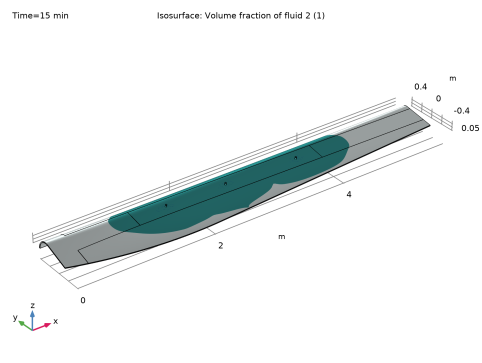
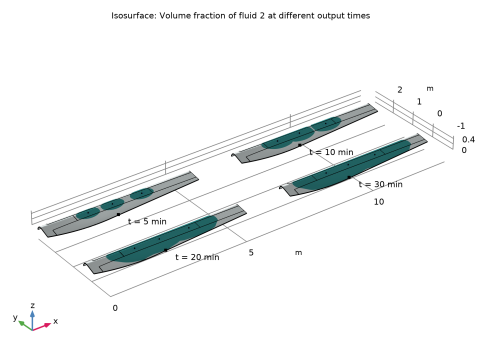
In the Settings window for 3D Plot Group, type Volume Fraction of Fluid 2 - Array in the Label text field.
4
Click to expand the Plot Array section. Select the Enable checkbox.
5
From the Array shape list, choose Square.
Isosurface 1
1
In the Model Builder window, click Isosurface 1.
2
In the Settings window for Isosurface, click to expand the Plot Array section.
3
Locate the Data section. From the Dataset list, choose Study 1/Solution 1 (sol1).
4
From the Time (min) list, choose 5.
5
Locate the Plot Array section. Select the Manual indexing checkbox.
6
In the Row index text field, type 1.
Isosurface 2
1
Right-click Results > Volume Fraction of Fluid 2 - Array > Isosurface 1 and choose Duplicate.
2
In the Settings window for Isosurface, locate the Data section.
3
From the Time (min) list, choose 10.
4
Locate the Plot Array section. In the Column index text field, type 1.
Isosurface 1, Isosurface 2
1
In the Model Builder window, under Results > Volume Fraction of Fluid 2 - Array, Ctrl-click to select Isosurface 1 and Isosurface 2.
2
Isosurface 3
1
In the Settings window for Isosurface, locate the Data section.
2
From the Time (min) list, choose 20.
3
Locate the Plot Array section. In the Row index text field, type 0.
Isosurface 4
1
In the Model Builder window, click Isosurface 4.
2
In the Settings window for Isosurface, locate the Data section.
3
From the Time (min) list, choose 30.
4
Click the  Zoom Extents button in the Graphics toolbar.
5
Locate the Plot Array section. In the Row index text field, type 0.
6
In the Volume Fraction of Fluid 2 - Array toolbar, click  Plot.
Now add the annotations to the different plots within the plot array.
Volume Fraction of Fluid 2 - Array
In the Model Builder window, click Volume Fraction of Fluid 2 - Array.
Table Annotation 1
1
In the Volume Fraction of Fluid 2 - Array toolbar, click  More Plots and choose Table Annotation.
2
In the Settings window for Table Annotation, locate the Data section.
3
From the Source list, choose Local table.
4
Volume Fraction of Fluid 2 - Array
1
In the Model Builder window, click Volume Fraction of Fluid 2 - Array.
2
In the Settings window for 3D Plot Group, click to expand the Title section.
3
From the Title type list, choose Manual.
4
In the Title text area, type Isosurface: Volume fraction of fluid 2 at different output times.
5
Clear the Parameter indicator text field.
6
In the Volume Fraction of Fluid 2 - Array toolbar, click  Plot.
7
Click the  Zoom Extents button in the Graphics toolbar.