PDF

Homogenization of Non-Newtonian
Porous Media Flow
Introduction
Understanding the dynamics of non-Newtonian flow in porous media is crucial for a variety of scientific and industrial applications. Non-Newtonian fluids exhibit complex flow characteristics that depend on the shear rate. This makes their behavior in porous media — such as soil, rock, and engineered materials — particularly challenging to model and predict. Pore-scale modeling is an essential tool to capture these flow patterns and interactions at a microscopic level, and to find patterns that can be used to derive homogenized properties that can be used at the macroscale.
This model shows how to use pore-scale modeling of non-Newtonian flow through a porous structure to find homogenized quantities for modeling at the macroscopic scale. It also compares the results and proves that this is a valuable approach that can be carried on to other applications.
Model Definition
The modeling process starts with opening the model file from Analyzing Porous Structures on the Microscopic Scale in the Porous Media Module Application Library. This model (Figure 1) was used to compute the porosity εp and permeability κ (m2) of the porous structure. The results are listed in Table 1. These values are intrinsic values of the porous structure and do not depend on the fluid flow.
Figure 1: Results from the initial model for computing the porosity and permeability.
Describing non-Newtonian flow in porous media with mathematical models remains an active research area due to the complexity of these flows. No universally applicable model exists yet. The flow behavior in porous media strongly depends on pore geometry, and one approach to describe it uses the concept of an apparent shear rate. Unlike free non-Newtonian flow, where shear rate can be calculated directly from flow velocity, the apparent shear rate depends on pore geometry and fluid properties. Therefore, it must be determined experimentally or numerically for each configuration.
The apparent shear rate (1/s) is often assumed to take the following form (Ref. 1):
(1)
The term is called the normalized velocity with the velocity magnitude v.
The correction factor α can be assumed to be constant within a certain velocity range for a specific fluid, so it must be determined individually for each setup. The advantage of this approach is that well-known non-Newtonian fluid models can be used as they are. In this context, a Carreau fluid is used with an apparent viscosity of
(2)
The idea is now to compute the apparent viscosity at the pore scale using Darcy’s Law:
(3)
After rearranging Equation 2, compute the apparent shear rate:
(4)
Using a Least-Squares Fit function to fit Equation 1 to the computed values gives α, which then can be used for the Brinkman Equations on the macroscale.
εp
κ
μ0
μinf
λ
Results and Discussion
After computing the pore-scale non-Newtonian flow for different pressure drops, inspect the viscosity (Figure 2). The fluid’s shear-thinning characteristics are clearly visible, especially at high-pressure drops and high velocities. In narrow regions with higher velocities, the viscosity is low, while in areas with lower velocities, the viscosity is high.
.
Figure 2: Dynamic viscosity for inlet pressure of 10 Pa and 100 Pa.
With these results, the apparent shear rate is computed using Equation 4. The resulting values are then fitted using Equation 1 to find the correction factor α. Figure 3 shows that the linear relationship is a good approximation for the considered pressure range.
Figure 3: Least-square fitted data.
The value for α is approximately 3.24. With this, the homogenization is completed. To verify the results, a model using Brinkman Equations is set up and the results are compared. Figure 4 and Figure 5 show that the results using the homogenized approach match the ones from the pore scale very well.
Figure 4: Apparent shear rate.
Figure 5: Apparent viscosity.
Reference
1. N. Zamani, I. Bondino, R. Kaufmann, and A. Skauge, “Computation of polymer in-situ rheology using direct numerical simulation,” J. Pet. Sci. Eng., vol. 159, pp. 92–102, 2017.
Application Library path: Polymer_Flow_Module/Tutorials/homogenization_non_newtonian_porous
Modeling Instructions
Root
Start by opening the model pore_scale_flow_3d from the Porous Media Flow Module Application Library. If you have not installed the Application Library you can alternatively download the model from the COMSOL website.
Application Libraries
1
From the File menu, choose Application Libraries.
2
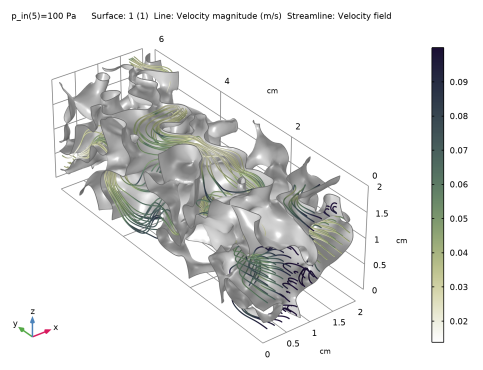
In the Application Libraries window, select Porous Media Flow Module > Fluid Flow > pore_scale_flow_3d in the tree.
3
Results
Velocity
1
In the Model Builder window, under Results click Velocity.
The model has been used to calculate the porosity and permeability of the porous structure. These values, which represent the intrinsic properties of the porous medium, now serve as inputs for the model. To utilize them throughout the whole model, create parameters based on the values provided in Table 1 under the Graphics window. Additionally, add parameters for the Carreau fluid.
Global Definitions
Parameters 1
1
In the Model Builder window, expand the Results > Tables node, then click Global Definitions > Parameters 1.
2
In the Settings window for Parameters, locate the Parameters section.
3
Component 1 (comp1)
In the Model Builder window, expand the Component 1 (comp1) node.
Creeping Flow (spf)
Fluid Properties 1
1
In the Model Builder window, expand the Component 1 (comp1) > Creeping Flow (spf) node, then click Fluid Properties 1.
2
In the Settings window for Fluid Properties, locate the Fluid Properties section.
3
Find the Constitutive relation subsection. From the list, choose Inelastic non-Newtonian.
4
From the Inelastic model list, choose Carreau.
Edit the material properties using the parameters.
Global Definitions
Material 1 (mat1)
1
In the Model Builder window, expand the Global Definitions > Materials node, then click Material 1 (mat1).
2
In the Settings window for Material, locate the Material Contents section.
3
Definitions
Variables 1
Add the expressions for the apparent viscosity and apparent shear rate to the table using Equation 3 and Equation 4 respectively.
1
In the Model Builder window, expand the Component 1 (comp1) > Definitions node, then click Variables 1.
2
In the Settings window for Variables, locate the Variables section.
3
Creeping Flow (spf)
Inlet 1
1
In the Model Builder window, under Component 1 (comp1) > Creeping Flow (spf) click Inlet 1.
2
In the Settings window for Inlet, locate the Boundary Condition section.
3
4
Locate the Pressure Conditions section. Click to select the p0 text field. Right-click and choose Create Parameter.
5
In the Create Parameter dialog, type p_in in the Name text field.
6
In the Expression text field, type 1[Pa].
7
In the Description text field, type Inlet pressure.
8
Add Study
1
In the Study toolbar, click  Add Study to open the Add Study window.
2
Go to the Add Study window.
3
Find the Studies subsection. In the Select Study tree, select General Studies > Stationary.
4
Click the Add Study button in the window toolbar.
5
In the Study toolbar, click  Add Study to close the Add Study window.
Study 2
Step 1: Stationary
1
In the Settings window for Stationary, click to expand the Study Extensions section.
2
Select the Auxiliary sweep checkbox.
3
4
5
6
In the Model Builder window, click Study 2.
7
In the Settings window for Study, locate the Study Settings section.
8
Clear the Generate default plots checkbox.
9
In the Study toolbar, click  Compute.
Reuse the velocity plot to visualize the viscosity. The streamlines color table currently indicates velocity magnitude, but switch it to show viscosity instead. To keep the original Velocity plot in the model, duplicate it first, then make the modifications.
Results
Viscosity
1
In the Model Builder window, right-click Velocity and choose Duplicate.
2
In the Settings window for 3D Plot Group, type Viscosity in the Label text field.
3
Locate the Data section. From the Dataset list, choose Study 2/Solution 2 (sol2).
Streamline 1
1
In the Model Builder window, expand the Viscosity node, then click Streamline 1.
2
In the Settings window for Streamline, locate the Coloring and Style section.
3
Find the Point style subsection. From the Type list, choose None.
4
Locate the Streamline Positioning section. In the Number text field, type 80.
Color Expression 1
1
In the Model Builder window, expand the Streamline 1 node, then click Color Expression 1.
2
In the Settings window for Color Expression, locate the Expression section.
3
In the Expression text field, type spf.mu.
4
Locate the Coloring and Style section. From the Color table list, choose Lichen.
5
In the Viscosity toolbar, click  Plot. Compare with Figure 2.
Next, compute the normalized velocity, apparent shear rate, and apparent viscosity as previously defined under Variables 1.
Global Evaluation 2
1
In the Results toolbar, click  Global Evaluation.
2
In the Settings window for Global Evaluation, locate the Data section.
3
From the Dataset list, choose Study 2/Solution 2 (sol2).
4
Locate the Expressions section. In the table, enter the following settings:
5
Clicknext to  Evaluate, then choose New Table.
Table 2
1
Go to the Table 2 window.
2
Click the Table Graph button in the window toolbar.
Results
Table Graph 1
1
In the Settings window for Table Graph, locate the Data section.
2
From the x-axis data list, choose u_out/sqrt(poro*kappa0) (1/s).
3
From the Plot columns list, choose Manual.
4
In the Columns list, select gamma_app (1/s).
Apparent Shear Rate vs. Normalized Velocity
1
In the Model Builder window, under Results click 1D Plot Group 4.
2
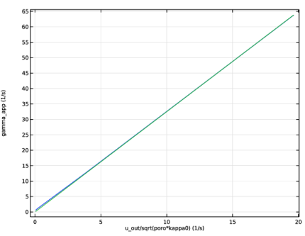
In the Settings window for 1D Plot Group, type Apparent Shear Rate vs. Normalized Velocity in the Label text field.
3
In the Apparent Shear Rate vs. Normalized Velocity toolbar, click  Plot.
Next, set up a Least-Squares Fit function to find α in Equation 1.
Global Definitions
Least-Squares Fit 1 (lsq1_fun1)
1
In the Home toolbar, click  Functions and choose Global > Least-Squares Fit.
2
In the Settings window for Least-Squares Fit, locate the Data section.
3
From the Data source list, choose Result table.
4
From the Result table list, choose Table 2.
5
Locate the Data Column Settings section. In the table, enter the following settings:
6
Locate the Parameters section. Click  Clear Table.
7
Locate the Data Column Settings section. In the table, click to select the cell at row number 3 and column number 3.
8
In the Expression text field, type alpha*x1.
9
Locate the Parameters section. In the table, enter the following settings:
10
Click  Fit Parameters.
11
Add Component
In the Model Builder window, right-click the root node and choose Add Component > 3D.
Geometry 2
Block 1 (blk1)
1
In the Geometry toolbar, click  Block.
2
In the Settings window for Block, locate the Size and Shape section.
3
In the Width text field, type 2[cm].
4
In the Depth text field, type 6[cm].
5
In the Height text field, type 2[cm].
Add Physics
1
In the Physics toolbar, click  Add Physics to open the Add Physics window.
2
Go to the Add Physics window.
3
In the tree, select Fluid Flow > Porous Media and Subsurface Flow > Brinkman Equations (br).
4
Find the Physics interfaces in study subsection. In the table, clear the Solve checkboxes for Study 1 and Study 2.
5
Click the Add to Component 2 button in the window toolbar.
6
In the Physics toolbar, click  Add Physics to close the Add Physics window.
Brinkman Equations (br)
Fluid 1
1
In the Settings window for Fluid, locate the Fluid Properties section.
2
From the ρ list, choose User defined. In the associated text field, type rho_f.
3
Find the Constitutive relation subsection. From the list, choose Inelastic non-Newtonian.
4
From the Inelastic model list, choose Carreau.
5
Find the Apparent shear rate subsection. In the α text field, type lsq1.alpha.
Materials
Material Link 2 (matlnk2)
1
In the Model Builder window, under Component 2 (comp2) right-click Materials and choose More Materials > Material Link.
2
In the Settings window for Material Link, locate the Link Settings section.
3
Click  Go to Material.
Global Definitions
Material 1 (mat1)
1
In the Model Builder window, under Global Definitions > Materials click Material 1 (mat1).
2
In the Settings window for Material, locate the Material Contents section.
3
Brinkman Equations (br)
In the Model Builder window, under Component 2 (comp2) click Brinkman Equations (br).
Inlet 1
1
In the Physics toolbar, click  Boundaries and choose Inlet.
2
3
In the Settings window for Inlet, locate the Boundary Condition section.
4
5
Locate the Pressure Conditions section. In the p0 text field, type p_in.
Outlet 1
1
In the Physics toolbar, click  Boundaries and choose Outlet.
2
Symmetry 1
1
In the Physics toolbar, click  Boundaries and choose Symmetry.
2
Define variables which are later used to compare the porous approach with the pore-scale modeling.
Definitions (comp2)
Average 3 (aveop3)
1
In the Definitions toolbar, click  Nonlocal Couplings and choose Average.
2
In the Settings window for Average, locate the Source Selection section.
3
From the Selection list, choose All domains.
Variables 2
1
In the Model Builder window, right-click Definitions and choose Variables.
2
In the Settings window for Variables, locate the Variables section.
3
Add Study
1
In the Study toolbar, click  Add Study to open the Add Study window.
2
Go to the Add Study window.
3
Find the Studies subsection. In the Select Study tree, select General Studies > Stationary.
4
Find the Physics interfaces in study subsection. In the table, clear the Solve checkbox for Creeping Flow (spf).
5
Click the Add Study button in the window toolbar.
6
In the Study toolbar, click  Add Study to close the Add Study window.
Study 3
Step 1: Stationary
1
In the Settings window for Stationary, locate the Study Extensions section.
2
Select the Auxiliary sweep checkbox.
3
4
5
In the Model Builder window, click Study 3.
6
In the Settings window for Study, locate the Study Settings section.
7
Clear the Generate default plots checkbox.
8
In the Study toolbar, click  Compute.
Results
Global Evaluation 3
1
In the Model Builder window, under Results > Derived Values right-click Global Evaluation 2 and choose Duplicate.
2
In the Settings window for Global Evaluation, locate the Data section.
3
From the Dataset list, choose Study 3/Solution 3 (4) (sol3).
4
Clicknext to  Evaluate, then choose New Table.
Table Graph 2
1
In the Model Builder window, under Results > Apparent Shear Rate vs. Normalized Velocity right-click Table Graph 1 and choose Duplicate.
2
In the Settings window for Table Graph, locate the Data section.
3
From the Table list, choose Table 3.
4
In the Apparent Shear Rate vs. Normalized Velocity toolbar, click  Plot. Compare with Figure 4.
Apparent Viscosity vs. Normalized Velocity
1
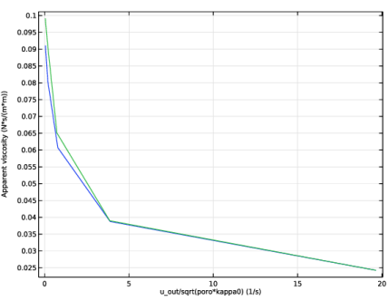
In the Model Builder window, right-click Apparent Shear Rate vs. Normalized Velocity and choose Duplicate.
2
In the Settings window for 1D Plot Group, type Apparent Viscosity vs. Normalized Velocity in the Label text field.
Table Graph 1
1
In the Model Builder window, expand the Apparent Viscosity vs. Normalized Velocity node, then click Table Graph 1.
2
In the Settings window for Table Graph, locate the Data section.
3
In the Columns list, select Apparent viscosity (N*s/(m*m)).
Table Graph 2
1
In the Model Builder window, click Table Graph 2.
2
In the Settings window for Table Graph, locate the Data section.
3
In the Columns list, select Apparent viscosity (N*s/(m*m)).
4
In the Apparent Viscosity vs. Normalized Velocity toolbar, click  Plot. Compare with Figure 5.