PDF

Radio Frequency Quadrupole Ion Trap
Introduction
A radio frequency quadrupole ion trap utilizes a radio frequency quadrupole (RFQ) in order to trap an ion beam. A continuous high energy ion beam is first cooled and converted into a spatially confined bunch, which can then be released with minimal heating of the beam (Ref. 1). The device is also commonly referred to as a Paul trap where an oscillating AC voltage is used to contain the beam radially. The axial confinement of the particles is achieved by using a DC voltage along the length of the quadrupole designed to create a potential well that can contain the beam.
The RFQ is often used to guide particle beams with kinetic energies in the order of 10–100 eV. In order to efficiently trap these particles, the kinetic energies are reduced through a process called buffer-gas cooling. The high energy charged beam is made to pass through a buffer gas, often consisting of a low molecular mass inert gas such as He or Ar. The highly energetic ions undergo elastic collisions with the light and slow moving buffer gas molecules, thus reducing the overall kinetic energy of the particle beam. The RF electric fields help contain the collisional scattering in the radial direction.
The device can be operated in two configurations: trapping and extraction. In the trapping configuration, the axial DC voltage contains a minima which helps in trapping the cooled beam. The cooled beam is therefore collected near the minima as a bunch of particles. This bunch can then be extracted by altering the DC voltage to help guide the beam out of the quadrupole. This two-stage operation thus allows for a continuous beam to be converted to a pulsed beam.
Model Definition
The geometry consists of four parallel cylindrical rods placed along a fixed radius as shown in Figure 1. An outer case is present to bound the particle trajectories. The particle beam enters the quadrupole from one end of the device and can exit through any surface of the case.
A positive potential of magnitude VAC is applied to the north and south rods, while a negative potential of the same magnitude is applied to the east and west rods. The motion of a charged particle in a RFQ is determined by the Mathieu equation whose solutions outline the stability region for the particle motion. In this model, the geometry and voltage parameters are chosen to ensure the stable motion of the charged particles (ions).
Once the ions enter the RFQ, they undergo elastic collisions with the buffer gas which helps in reducing the kinetic energy of the ions, thus cooling the beam. The ions in this model are composed of Cs+ ions which undergo collisions with He atoms. The He atoms are modeled as a background gas and thus their motion is not explicitly modeled. The collisional interactions are modeled using the Collisions node with an Elastic subnode. This approach utilizes a Monte-Carlo approach for modeling the collisions whereby at each time step taken by the solver, a He atom is sampled from a Maxwell–Boltzmann distribution. The probability of collision is then computed for each ion and if a collision is deemed to occur, an elastic collision is modeled where the energy of the collision is conserved. The collision frequency depends on the number density of the gas, the collision cross section, and the relative velocity between the ion and the background gas atom. This model uses the Hard Sphere collision model where the collision cross section is constant and independent of the relative velocity. The gas pressure chosen in this model is 6 Pa.
Figure 1: Model geometry of a radio frequency quadrupole ion trap.
This model demonstrates the two-stage operation of the RFQ ion trap. In the first stage, a trapping DC potential is used in addition to the buffer gas cooling in order to trap and bunch the ions spatially. Once the ion beam is cooled and bunched, the DC potential is altered to the extraction mode which allows the cooled beam to exit the RFQ. Thus a continuous ion beam can be converted to a pulsed beam. The two potentials are shown in Figure 2.
Figure 2: Trapping and extraction configuration of the axial DC potentials. The unlabeled line represents the beam trajectory as it is cooled and trapped.
The ion beam is released into the domain using the Particle Beam feature. In order to release a continuous beam, 20 ions are released at a time interval equal to 1/20 of the RF cycle. Ions are released up to five cycles such that a total of 2000 ions are released. The ions are released with an initial longitudinal kinetic energy of 60 eV. Two Electric Force features are used in this model to account for the electric forces resulting from the AC and DC voltages.
Notes on COMSOL Implementation
The model uses three physics interfaces: Electrostatics, Electric Currents and Charged Particle Tracing. The model is solved in four steps.
First the Electrostatics (using the trapping potential), Electric Currents interfaces are used to compute the DC and AC electric fields respectively. These fields are then coupled to the Charged Particle Tracing interface to compute the particle motion under the influence of the electric forces and collisions with the buffer gas.
Once the ion beams are cooled and bunched near the potential minima, the DC voltage in the Electrostatics interface is altered to the extraction potential. The Electrostatics and the Electric Currents interfaces are again used to compute the new DC and AC electric fields. Finally, the Charged Particle Tracing interface utilizes the particle positions and velocities from the previous study as the initial conditions to compute the particle trajectories under the influence of the newly computed electric fields and buffer gas collisions. In order to enable this initialization of the particle properties from a previous study, the Store particle status data checkbox must be selected in the Additional Variables section in the settings for the Charged Particle Tracing interface.
Results and Discussion
The particle positions at the end of the trapping stage (300 μs) are plotted in Figure 3. The particles are colored by their overall kinetic energy (in eV). The ion beam entered the domain with a longitudinal kinetic energy of 60 eV. Therefore, it is clear that the beam has been significantly cooled. Furthermore, a continuous beam of ions have been collected and bunched as can be seen by the narrow longitudinal spread of the ions.
Figure 3: Positions of the cooled and bunched ion beam.
As the beam cools and encounters the potential barrier, it is repulsed and thus the beam oscillates axially and asymptotically settles near the potential minima (Ref. 1). This is schematically shown in Figure 2 where the unlabeled line represents the beam’s average axial position (x-axis) as a function of time (y-axis). The time is scaled so that the plot superimposes onto the trapping potential. This line is colored by its average kinetic energy.
Figure 4: Transverse beam profiles at various solution times (annotated in μs).
The repeated ion-gas collisions reduces the kinetic energy of the ions and the RF voltages constrain the radial diffusion of the particles. As a result, the radial spread of the particles is greatly reduced. This is visualized in Figure 4 where the transverse beam profiles are plotted at different solution times. The radial spread of the ion beam clearly diminishes as a function of time. A similar effect is also observed in the transverse phase portrait plots of the position-velocity phase space as shown in Figure 5.
Figure 5: Transverse phase portraits showing the position-velocity phase space of the beam at various solution times (annotated in μs).
Finally, the cooled and bunched beam is released by altering the DC voltage to the extraction mode and the particle trajectories of this ion bunch are plotted in Figure 6. It can be seen that the particles promptly exit the domain and the heating of the beam is minimal.
Figure 6: Particle trajectories under the influence of the extraction potential and buffer-gas cooling.
References
1. Brunner, T., M. J. Smith, M. Brodeur, S. Ettenauer, A. T. Gallant, Vanessa V. Simon, A. Chaudhuri et al. "TITAN's digital RFQ ion beam cooler and buncher, operation and performance." Nuclear Instruments and Methods in Physics Research Section A: Accelerators, Spectrometers, Detectors and Associated Equipment 676 (2012): 32-43.
Application Library path: Particle_Tracing_Module/Charged_Particle_Tracing/rfq_ion_trap
Modeling Instructions
From the File menu, choose New.
New
In the New window, click  Model Wizard.
Model Wizard
1
In the Model Wizard window, click  3D.
2
In the Select Physics tree, select AC/DC > Electric Fields and Currents > Electrostatics (es).
3
Click Add.
4
In the Select Physics tree, select AC/DC > Electric Fields and Currents > Electric Currents (ec).
5
Click Add.
6
In the Select Physics tree, select AC/DC > Particle Tracing > Charged Particle Tracing (cpt).
7
Click Add.
8
Click  Study.
9
In the Select Study tree, select Empty Study.
10
Global Definitions
Parameters 1
Load the model parameters from a file.
1
In the Model Builder window, under Global Definitions click Parameters 1.
2
In the Settings window for Parameters, locate the Parameters section.
3
Click  Load from File.
4
Definitions
Piecewise 1 (pw1)
1
In the Definitions toolbar, click  Piecewise.
2
In the Settings window for Piecewise, type trap_pot in the Function name text field.
3
Locate the Definition section. From the Smoothing list, choose Continuous second derivative.
4
In the Size of transition zone text field, type L_rod/4.
5
Find the Intervals subsection. In the table, enter the following settings:
6
Locate the Units section. In the Arguments text field, type m.
7
In the Function text field, type V.
8
In the Model Builder window, under Component 1 (comp1) > Definitions click Piecewise 1 (trap_pot).
9
Click  Create Plot.
Analytic 1 (an1)
1
In the Definitions toolbar, click  Analytic.
2
In the Settings window for Analytic, type ext_pot in the Function name text field.
3
Locate the Definition section. In the Expression text field, type V1/x_min*x.
4
Locate the Units section. In the table, enter the following settings:
5
Locate the Plot Parameters section. In the table, enter the following settings:
Now plot the two functions to visualize the trapping and extraction potentials.
Results
Axial DC voltages
1
In the Model Builder window, under Results click 1D Plot Group 1.
2
In the Settings window for 1D Plot Group, type Axial DC voltages in the Label text field.
Function 1
1
In the Model Builder window, expand the Axial DC voltages node, then click Function 1.
2
In the Settings window for Function, locate the y-Axis Data section.
3
In the Description text field, type Trapping Potential.
4
Locate the x-Axis Data section. From the Unit list, choose mm.
5
In the Description text field, type x.
6
In the Upper bound text field, type 250.
7
Click to expand the Coloring and Style section. Find the Line style subsection. From the Line list, choose Cycle.
8
From the Width list, choose 3.
9
Click to expand the Legends section. Select the Show legends checkbox.
10
In the Axial DC voltages toolbar, click  Plot.
Grid 1D 1
1
In the Model Builder window, expand the Results > Datasets node, then click Grid 1D 1.
2
In the Settings window for Grid 1D, locate the Data section.
3
From the Function list, choose All.
Function 2
1
In the Model Builder window, under Results > Axial DC voltages right-click Function 1 and choose Duplicate.
2
In the Settings window for Function, locate the y-Axis Data section.
3
In the Expression text field, type comp1.ext_pot(x).
4
In the Description text field, type Extraction Potential.
Axial DC voltages
1
In the Model Builder window, click Axial DC voltages.
2
In the Settings window for 1D Plot Group, locate the Plot Settings section.
3
Select the x-axis label checkbox.
4
Select the y-axis label checkbox. In the associated text field, type Axial voltage (V).
5
Click to expand the Title section. From the Title type list, choose None.
6
In the Axial DC voltages toolbar, click  Plot. The trapping and extraction potentials should resemble Figure 2.
Add Material
1
In the Materials toolbar, click  Add Material to open the Add Material window.
2
Go to the Add Material window.
3
In the tree, select Built-in > Perfect vacuum.
4
Click the Add to Component button in the window toolbar.
5
In the Materials toolbar, click  Add Material to close the Add Material window.
Geometry 1
Work Plane 1 (wp1)
1
In the Geometry toolbar, click  Work Plane.
2
In the Settings window for Work Plane, locate the Plane Definition section.
3
From the Plane list, choose yz-plane.
Work Plane 1 (wp1) > Plane Geometry
In the Model Builder window, click Plane Geometry.
Work Plane 1 (wp1) > Circle 1 (c1)
1
In the Work Plane toolbar, click  Circle.
2
In the Settings window for Circle, locate the Size and Shape section.
3
In the Radius text field, type r_rod.
4
Locate the Position section. In the xw text field, type r_rod+r0.
5
Click  Build Selected.
Work Plane 1 (wp1) > Circle 2 (c2)
1
Right-click Component 1 (comp1) > Geometry 1 > Work Plane 1 (wp1) > Plane Geometry > Circle 1 (c1) and choose Duplicate.
2
In the Settings window for Circle, locate the Position section.
3
In the xw text field, type -(r_rod+r0).
Work Plane 1 (wp1) > Circle 3 (c3)
1
Right-click Component 1 (comp1) > Geometry 1 > Work Plane 1 (wp1) > Plane Geometry > Circle 2 (c2) and choose Duplicate.
2
In the Settings window for Circle, locate the Position section.
3
In the xw text field, type 0.
4
In the yw text field, type -(r_rod+r0).
Work Plane 1 (wp1) > Circle 4 (c4)
1
Right-click Component 1 (comp1) > Geometry 1 > Work Plane 1 (wp1) > Plane Geometry > Circle 3 (c3) and choose Duplicate.
2
In the Settings window for Circle, locate the Position section.
3
In the yw text field, type r_rod+r0.
4
In the Home toolbar, click  Build All.
5
Click the  Zoom Extents button in the Graphics toolbar.
Extrude 1 (ext1)
1
In the Model Builder window, under Component 1 (comp1) > Geometry 1 right-click Work Plane 1 (wp1) and choose Extrude.
2
In the Settings window for Extrude, locate the Distances section.
3
4
Click  Build Selected.
Cylinder 1 (cyl1)
1
In the Geometry toolbar, click  Cylinder.
2
In the Settings window for Cylinder, locate the Size and Shape section.
3
In the Radius text field, type r_case.
4
In the Height text field, type L_rod.
5
Locate the Axis section. From the Axis type list, choose x-axis.
Difference 1 (dif1)
1
In the Geometry toolbar, click  Booleans and Partitions and choose Difference.
2
3
In the Settings window for Difference, locate the Difference section.
4
Click to select the  Activate Selection toggle button for Objects to subtract.
5
6
Click  Build Selected.
Form Union (fin)
1
In the Geometry toolbar, click  Build All.
2
Click the  Zoom Extents button in the Graphics toolbar.
Definitions
All rods
1
In the Definitions toolbar, click  Explicit.
2
In the Settings window for Explicit, type All rods in the Label text field.
3
Locate the Input Entities section. From the Geometric entity level list, choose Boundary.
4
Select the Group by continuous tangent checkbox.
5
y-pair
1
In the Definitions toolbar, click  Explicit.
2
In the Settings window for Explicit, type y-pair in the Label text field.
3
Locate the Input Entities section. From the Geometric entity level list, choose Boundary.
4
Select the Group by continuous tangent checkbox.
5
z-pair
1
In the Definitions toolbar, click  Explicit.
2
In the Settings window for Explicit, type z-pair in the Label text field.
3
Locate the Input Entities section. From the Geometric entity level list, choose Boundary.
4
Select the Group by continuous tangent checkbox.
5
Electrostatics (es)
Electric Potential 1
1
In the Model Builder window, expand the Component 1 (comp1) > Electrostatics (es) node.
2
Right-click Electrostatics (es) and choose Electric Potential.
3
In the Settings window for Electric Potential, locate the Electric Potential section.
4
In the V0 text field, type trap_pot(x).
5
Locate the Boundary Selection section. From the Selection list, choose All rods.
Electric Currents (ec)
1
In the Model Builder window, under Component 1 (comp1) click Electric Currents (ec).
2
In the Physics toolbar, click  Boundaries and choose Electric Potential.
1
In the Settings window for Electric Potential, locate the Boundary Selection section.
2
From the Selection list, choose z-pair.
3
Locate the Electric Potential section. In the V0 text field, type V_AC.
Electric Potential 2
1
In the Physics toolbar, click  Boundaries and choose Electric Potential.
2
In the Settings window for Electric Potential, locate the Boundary Selection section.
3
From the Selection list, choose y-pair.
4
Locate the Electric Potential section. In the V0 text field, type -V_AC.
Mesh 1
1
In the Model Builder window, under Component 1 (comp1) click Mesh 1.
2
In the Settings window for Mesh, locate the Physics-Controlled Mesh section.
3
From the Element size list, choose Extra fine.
4
Click  Build All.
First solve for the electric fields. The Electrostatics (es) physics interface will be solved using a Stationary study step, while the Electric Currents (ec) physics interface will be solved using a Time Dependent study step
Study 1: Electric Fields
1
In the Model Builder window, click Study 1.
2
In the Settings window for Study, type Study 1: Electric Fields in the Label text field.
Step 1: Stationary
1
In the Study toolbar, click  Study Steps and choose Stationary > Stationary.
2
In the Settings window for Stationary, locate the Physics and Variables Selection section.
3
In the Solve for column of the table, under Component 1 (comp1), clear the checkbox for Electric Currents (ec).
Step 2: Frequency Domain
1
In the Study toolbar, click  Study Steps and choose Frequency Domain > Frequency Domain.
2
In the Settings window for Frequency Domain, locate the Study Settings section.
3
In the Frequencies text field, type f.
4
Locate the Physics and Variables Selection section. In the Solve for column of the table, under Component 1 (comp1), clear the checkbox for Electrostatics (es).
5
Click to expand the Values of Dependent Variables section. Find the Values of variables not solved for subsection. From the Settings list, choose User controlled.
6
From the Method list, choose Solution.
7
From the Study list, choose Study 1: Electric Fields, Stationary.
8
In the Study toolbar, click  Compute.
Now that the electric fields are solved for, set up the Charged Particle Tracing (cpt) physics interface to compute the particle trajectories.
Charged Particle Tracing (cpt)
1
In the Model Builder window, under Component 1 (comp1) click Charged Particle Tracing (cpt).
2
In the Settings window for Charged Particle Tracing, locate the Additional Variables section.
3
Select the Store particle status data checkbox.
Selecting this checkbox is necessary for utilizing the particle trajectories of one study step as the initial conditions for another study step.
Wall 1
1
In the Model Builder window, under Component 1 (comp1) > Charged Particle Tracing (cpt) click Wall 1.
2
In the Settings window for Wall, locate the Wall Condition section.
3
From the Wall condition list, choose Disappear.
Particle Properties 1
1
In the Model Builder window, click Particle Properties 1.
2
In the Settings window for Particle Properties, locate the Particle Mass section.
3
In the mp text field, type mass_ion.
4
Locate the Charge Number section. In the Z text field, type 1.
Use the particle beam release feature to release a continuous beam of charged particles during the first five cycles of the oscillating voltage.
Particle Beam 1
1
In the Physics toolbar, click  Boundaries and choose Particle Beam.
2
3
In the Settings window for Particle Beam, locate the Release Times section.
4
In the Release times text field, type range(0,(5*T_osc-0)/99,5*T_osc).
5
Locate the Initial Position section. In the N text field, type 20.
6
Locate the Initial Transverse Velocity section. From the Transverse velocity distribution specification list, choose Specify phase space ellipse dimensions.
7
In the xm text field, type r_in.
8
Locate the Initial Longitudinal Velocity section. In the E text field, type E_in.
Electric Force 1
1
In the Physics toolbar, click  Domains and choose Electric Force.
2
3
In the Settings window for Electric Force, locate the Electric Force section.
4
From the E list, choose Electric field (es/fsp1).
Electric Force 2
1
In the Physics toolbar, click  Domains and choose Electric Force.
2
3
In the Settings window for Electric Force, locate the Electric Force section.
4
From the E list, choose Electric field (ec/cucn1).
5
Locate the Advanced Settings section. From the Time dependence of field list, choose Time harmonic.
Collisions 1
1
In the Physics toolbar, click  Domains and choose Collisions.
2
3
In the Settings window for Collisions, locate the Fluid Properties section.
4
In the Nd text field, type nd.
5
In the Mg text field, type 2[amu]*N_A_const.
6
In the T text field, type Tgas.
Elastic 1
In the Physics toolbar, click  Attributes and choose Elastic.
Outlet 1
1
In the Physics toolbar, click  Boundaries and choose Outlet.
2
Now add another study to compute the particle trajectories utilizing the previously computed electric fields.
Add Study
1
In the Home toolbar, click  Add Study to open the Add Study window.
2
Go to the Add Study window.
3
Find the Studies subsection. In the Select Study tree, select General Studies > Time Dependent.
4
Find the Physics interfaces in study subsection. In the table, clear the Solve checkboxes for Electrostatics (es) and Electric Currents (ec).
5
Click the Add Study button in the window toolbar.
6
In the Home toolbar, click  Add Study to close the Add Study window.
Study 2: Particle Tracing - Trapping Potential
In the Settings window for Study, type Study 2: Particle Tracing - Trapping Potential in the Label text field.
Step 1: Time Dependent
1
In the Model Builder window, under Study 2: Particle Tracing - Trapping Potential click Step 1: Time Dependent.
2
In the Settings window for Time Dependent, locate the Study Settings section.
3
From the Time unit list, choose µs.
4
In the Output times text field, type range(0,5.0,300).
5
Click to expand the Values of Dependent Variables section. Find the Values of variables not solved for subsection. From the Settings list, choose User controlled.
6
From the Method list, choose Solution.
7
From the Study list, choose Study 1: Electric Fields, Frequency Domain.
The modeling of the ion-gas collisions requires that the time steps taken by the solver be less than the mean collision time. Therefore, a fixed time step of 1e-8 s is utilized in this study.
Solution 3 (sol3)
1
In the Study toolbar, click  Show Default Solver.
2
In the Model Builder window, expand the Solution 3 (sol3) node, then click Time-Dependent Solver 1.
3
In the Settings window for Time-Dependent Solver, click to expand the Time Stepping section.
4
From the Steps taken by solver list, choose Manual.
5
In the Time step text field, type 1e-8.
6
In the Study toolbar, click  Compute.
Results
Particle Trajectories - Trapping Potential
In the Settings window for 3D Plot Group, type Particle Trajectories - Trapping Potential in the Label text field.
Particle Trajectories 1
1
In the Model Builder window, expand the Particle Trajectories - Trapping Potential node, then click Particle Trajectories 1.
2
In the Settings window for Particle Trajectories, locate the Coloring and Style section.
3
Find the Point style subsection.
4
Select the Radius scale factor checkbox. In the associated text field, type 0.25.
5
In the Particle Trajectories - Trapping Potential toolbar, click  Plot.
Color Expression 1
1
In the Model Builder window, expand the Particle Trajectories 1 node, then click Color Expression 1.
2
In the Settings window for Color Expression, locate the Expression section.
3
In the Expression text field, type cpt.Ep.
4
From the Unit list, choose eV.
5
In the Particle Trajectories - Trapping Potential toolbar, click  Plot.
The particle trajectories at the last time step should resemble Figure 3.
Animation 1
1
In the Particle Trajectories - Trapping Potential toolbar, click  Animation and choose Player.
2
In the Settings window for Animation, locate the Frames section.
3
From the Frame selection list, choose All.
4
Click the  Play button in the Graphics toolbar.
It is clear that the collisions with the Ar gas diminish the beam energy, and the shape of the axial potential causes the cooled beam to be trapped near the well. This can also be visualized by superimposing the average axial position of the beam as a function of time over the trapping potential.
Axial DC voltages
In the Model Builder window, under Results click Axial DC voltages.
Global 1
1
In the Axial DC voltages toolbar, click  Global.
2
In the Settings window for Global, locate the Data section.
3
From the Dataset list, choose Particle 1.
4
Locate the y-Axis Data section. In the table, enter the following settings:
The time parameter is scaled so as to fit neatly over the trapping potential.
5
Locate the x-Axis Data section. From the Parameter list, choose Expression.
6
In the Expression text field, type cpt.ave(qx).
7
From the Unit list, choose mm.
8
Click to expand the Coloring and Style section. From the Width list, choose 3.
9
Click to expand the Legends section. Clear the Show legends checkbox.
10
In the Axial DC voltages toolbar, click  Plot.
Color Expression 1
1
In the Axial DC voltages toolbar, click  Color Expression.
2
In the Settings window for Color Expression, locate the Expression section.
3
In the Expression text field, type cpt.Epave.
4
From the Unit list, choose eV.
5
Locate the Coloring and Style section. From the Color table list, choose Thermal.
Axial DC voltages
1
In the Model Builder window, under Results click Axial DC voltages.
2
In the Settings window for 1D Plot Group, locate the Axis section.
3
Select the Manual axis limits checkbox.
4
In the x minimum text field, type 0.
5
In the x maximum text field, type 250.
6
In the y minimum text field, type -12.
7
In the y maximum text field, type 10.
8
Locate the Color Legend section. Select the Show maximum and minimum values checkbox.
9
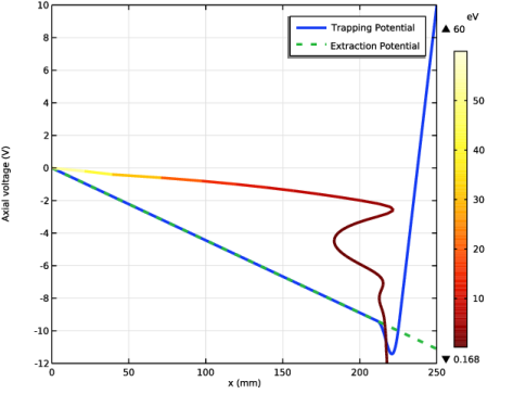
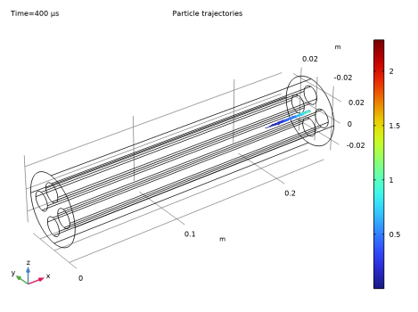
Select the Show units checkbox. The plot demonstrates the trapping of the beam and should resemble Figure 2.
Beam Profile
1
In the Results toolbar, click  1D Plot Group.
2
In the Settings window for 1D Plot Group, type Beam Profile in the Label text field.
3
Locate the Data section. From the Dataset list, choose Particle 1.
4
From the Time selection list, choose Interpolated.
5
In the Times (µs) text field, type 20.
Particle 1
1
In the Beam Profile toolbar, click  More Plots and choose Particle.
2
In the Settings window for Particle, locate the y-Axis Data section.
3
In the Expression text field, type qz.
4
From the Unit list, choose mm.
5
Locate the x-Axis Data section. From the Parameter list, choose Expression.
6
In the Expression text field, type qy.
7
From the Unit list, choose mm.
8
Click to expand the Coloring and Style section. Find the Line style subsection. From the Line list, choose None.
9
Find the Line markers subsection. From the Marker list, choose Circle.
Beam Profile
1
In the Model Builder window, click Beam Profile.
2
In the Settings window for 1D Plot Group, locate the Axis section.
3
Select the Manual axis limits checkbox.
4
In the x minimum text field, type -5.
5
In the x maximum text field, type 5.
6
In the y minimum text field, type -5.
7
In the y maximum text field, type 5.
8
Locate the Title section. From the Title type list, choose None.
9
In the Beam Profile toolbar, click  Plot.
Plot the beam profile at different solution times by selecting values from the Time (s) list. The beam profiles at different solution times are shown in Figure 4.
Transverse Phase Space
1
Right-click Beam Profile and choose Duplicate.
2
In the Settings window for 1D Plot Group, type Transverse Phase Space in the Label text field.
3
Locate the Data section. In the Times (µs) text field, type 20.
Particle 1
1
In the Model Builder window, expand the Transverse Phase Space node, then click Particle 1.
2
In the Settings window for Particle, locate the y-Axis Data section.
3
In the Expression text field, type cpt.vy.
4
From the Unit list, choose km/s. km/s is equivalent to the convenient scale of mm/μs.
5
In the Transverse Phase Space toolbar, click  Plot.
Plot the transverse phase portraits at different solution times by selecting values from the Time (s) list. The transverse phase portraits at different solution times are shown in Figure 5.
Now that the particles have been cooled and bunched together, alter the DC voltage to the extraction mode in order to release the cooled ions.
Electrostatics (es)
Electric Potential 1
1
In the Model Builder window, under Component 1 (comp1) > Electrostatics (es) click Electric Potential 1.
2
In the Settings window for Electric Potential, locate the Electric Potential section.
3
In the V0 text field, type ext_pot(x).
Study 1: Electric Fields
In the Study toolbar, click  Compute.
Add a new study to compute the particle trajectories under the influence of the extraction potential. This new study step will utilize the solution from Study 2 to initialize the particle position and velocities.
Add Study
1
In the Home toolbar, click  Add Study to open the Add Study window.
2
Go to the Add Study window.
3
Find the Studies subsection. In the Select Study tree, select General Studies > Time Dependent.
4
Find the Physics interfaces in study subsection. In the table, clear the Solve checkboxes for Electrostatics (es) and Electric Currents (ec).
5
Click the Add Study button in the window toolbar.
6
In the Home toolbar, click  Add Study to close the Add Study window.
Study 3: Particle Tracing - Extraction Potential
In the Settings window for Study, type Study 3: Particle Tracing - Extraction Potential in the Label text field.
Step 1: Time Dependent
1
In the Model Builder window, under Study 3: Particle Tracing - Extraction Potential click Step 1: Time Dependent.
2
In the Settings window for Time Dependent, locate the Study Settings section.
3
From the Time unit list, choose µs.
4
In the Output times text field, type range(300,10,400).
5
Locate the Values of Dependent Variables section. Find the Initial values of variables solved for subsection. From the Settings list, choose User controlled.
6
From the Method list, choose Solution.
7
From the Study list, choose Study 2: Particle Tracing - Trapping Potential, Time Dependent.
8
From the Time (µs) list, choose Last.
9
Find the Values of variables not solved for subsection. From the Settings list, choose User controlled.
10
From the Method list, choose Solution.
11
From the Study list, choose Study 1: Electric Fields, Frequency Domain.
Solution 4 (sol4)
1
In the Study toolbar, click  Show Default Solver.
2
In the Model Builder window, expand the Solution 4 (sol4) node, then click Time-Dependent Solver 1.
3
In the Settings window for Time-Dependent Solver, locate the Time Stepping section.
4
From the Steps taken by solver list, choose Manual.
5
In the Time step text field, type 1e-8.
6
In the Study toolbar, click  Compute.
Results
Particle Trajectories - Extraction potential
In the Settings window for 3D Plot Group, type Particle Trajectories - Extraction potential in the Label text field.
Particle Trajectories 1
1
In the Model Builder window, expand the Particle Trajectories - Extraction potential node, then click Particle Trajectories 1.
2
In the Settings window for Particle Trajectories, locate the Coloring and Style section.
3
Find the Line style subsection. From the Type list, choose Line.
4
Find the Point style subsection.
5
Select the Radius scale factor checkbox. In the associated text field, type 0.25.
Color Expression 1
1
In the Model Builder window, expand the Particle Trajectories 1 node, then click Color Expression 1.
2
In the Settings window for Color Expression, locate the Expression section.
3
In the Expression text field, type cpt.Ep.
4
From the Unit list, choose eV.
5
In the Particle Trajectories - Extraction potential toolbar, click  Plot.
The particle trajectories at the last time step should resemble Figure 6.
Animation 2
1
In the Model Builder window, under Results > Export right-click Animation 1 and choose Duplicate.
2
In the Settings window for Animation, locate the Scene section.
3
From the Subject list, choose Particle Trajectories - Extraction potential.
4
Click the  Play button in the Graphics toolbar.