COMSOL 6.3 - Inertial Focusing Between Two Parallel Walls

Inertial Focusing Between Two Parallel Walls

As neutrally buoyant particles are carried by a fluid in a cylindrical pipe, they are focused to a ring with a radius of approximately 0.6 times the pipe radius R. The ring of particles, which is caused by a combination of lift and drag forces, is sometimes called the Segré-Silberberg annulus in honor of Segré and Silberberg’s oft-cited observations of this effect (Ref. 1). The phenomenon by which particles migrate to this equilibrium position is called inertial focusing. Ho and Leal (Ref. 2) have derived expressions for the forces that cause a similar migration in a two-dimensional parabolic flow between two parallel walls.

In this example, the Particle Tracing for Fluid Flow interface is used to compute the trajectories of particles in a two-dimensional Poiseuille flow. This example uses built-in corrections to the lift force and drag force to account for the presence of the walls. A time dependent study demonstrates that the particles converge toward distances of 0.2D from either wall, where D is the distance between the walls, regardless of their initial positions.

Model Definition

The total force on the neutrally buoyant particles in a creeping flow consists of a drag force and lift force, since by definition the gravitational and buoyant forces cancel each other out. The particles experience a drag force given by Stokes’ law.

Where rp (SI unit m) is the particle radius, μ (SI unit Pa·s) is the fluid viscosity, u (SI unit m/s) is the fluid velocity, and v (SI unit m/s) is the particle velocity. The lift force is given by Ref. 2:

where

•

I (dimensionless) is the identity matrix,

•

n (dimensionless) is the wall normal at the nearest point on the reference wall,

•

D (SI unit: m) is the distance between the channel walls,

•

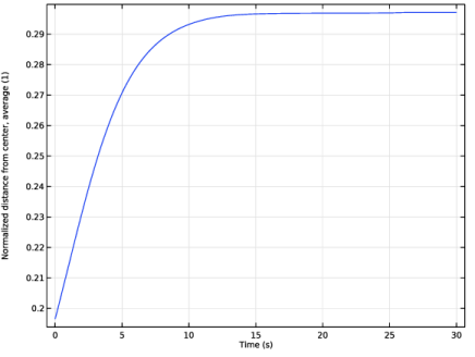
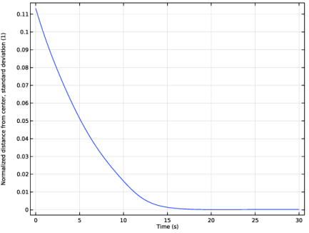
s is the normalized distance from the particle to the reference wall, divided by D so that 0 < s < 1 for particles in the channel

•

G1 and G2 are dimensionless functions of the normalized wall distance, given in Ref. 2. These functions are plotted in Figure 1 and Figure 2.

The lift force only acts in the direction perpendicular to the velocity of the fluid. The spherical particles are further assumed to be small compared to the channel width and rotationally rigid.

The velocity field u is first computed using the Laminar Flow physics interface, then coupled to the Particle Tracing for Fluid Flow physics interface using the node. The boundary condition is used to automatically compute a fully developed fluid velocity profile at the boundary. It is well-known that the fully developed velocity profile for the laminar flow of a Newtonian fluid between two parallel walls is parabolic, so in this example it would have also been possible to enter the analytic expression for the fluid velocity directly. However, the velocity has instead been computed using the Laminar Flow physics interface to demonstrate a workflow that is appropriate for a more general geometry.

Figure 1: The function G1(s) used to define the wall-induced lift force.

Figure 2: The function G2(s) used to define the wall-induced lift force.

Results and Discussion

The fluid velocity magnitude is plotted in Figure 3. Note that the plots are not drawn to scale; the channel length is much greater than the channel width. As expected for a laminar flow between two parallel walls, the velocity profile is parabolic.

The trajectories of the neutrally buoyant particles are plotted in Figure 4. The color expression is the y-component of the particle velocity in mm/s. All of the particles seem to approach equilibrium positions at distances of about 0.3D on either side of the channel center, where D is the channel width. Particles that are released near the center of the channel take more time to approach these equilibrium positions because they are released where the velocity gradient has the lowest magnitude, so the initial lift force is weaker.

The average and standard deviation of the normalized distance from the particles to the channel center are plotted in Figure 5 and Figure 6, respectively. This confirms that the equilibrium distance from the channel center is about 0.3D.

Figure 3: Parabolic fluid velocity profile in a channel bounded by two parallel walls.

Figure 4: Particle trajectories in the channel. The color expression is the y-component of the particle velocity in mm/s.

Figure 5: Average normalized distance of particles from the center of the channel.

Figure 6: Standard deviation of the normalized distance of particles from the center of the channel.

References

1. G. Segré, and A. Silberberg, “Behaviour of macroscopic rigid spheres in Poiseuille flow. Part 1. Determination of local concentration by statistical analysis of particle passages through crossed light beams,” J. Fluid Mech., vol. 14, pp. 115–135, 1962.

2. B.P. Ho and L.G. Leal. “Inertial migration of rigid spheres in two-dimensional unidirectional flows,” J. Fluid Mech., vol. 65, no. 2, pp. 365–400, 1974.

Particle_Tracing_Module/Fluid_Flow/inertial_focusing

Modeling Instructions

From the menu, choose .

New

In the window, click

Model Wizard

In the window, click

In the tree, select > > .

Click .

Click

In the tree, select > .

Click

Global Definitions

Parameters 1

In the window, under click .

In the window for , locate the section.

Click

Browse to the model’s Application Libraries folder and double-click the file inertial_focusing_parameters.txt.

Definitions

Variables 1

In the window, under right-click and choose .

In the window for , locate the section.

In the table, enter the following settings:


Name	Expression	Unit	Description
dn	abs(qy/d-0.5)		Normalized distance from center
dnave	fpt.ave(dn)		Normalized distance, average
dnstd	sqrt(fpt.ave(dn^2)-fpt.ave(dn)^2)		Normalized distance, standard deviation

These variables will be used during postprocessing to observe how the neutrally buoyant particles are focused by lift forces in the channel.

Axis

In the window, expand the > > node, then click .

In the window for , locate the section.

From the list, choose . This allows the geometry, which has an extremely high aspect ratio, to be viewed more easily.

Geometry 1

In the window, under click .

In the window for , locate the section.

From the list, choose .

Rectangle 1 (r1)

In the toolbar, click

In the window for , locate the section.

In the text field, type L.

In the text field, type d.

Click

Materials

Material 1 (mat1)

In the window, under right-click and choose .

In the window for , locate the section.

In the table, enter the following settings:


Property	Variable	Value	Unit	Property group
Density	rho	rhof	kg/m³	Basic
Dynamic viscosity	mu	muf	Pa·s	Basic

Use the Laminar Flow interface to compute the fluid velocity profile in the channel.

Laminar Flow (spf)

In the window, under click .

In the window for , click to expand the section.

From the list, choose . The lift force depends on the spatial derivatives of the fluid velocity components. Therefore, increasing the discretization order is required for accurate calculation of the particle trajectories.

Inlet 1

In the toolbar, click

and choose .

Select Boundary 1 only.

In the window for , locate the section.

From the list, choose .

Locate the section. In the Uav text field, type Vav.

Outlet 1

In the toolbar, click

and choose .

Select Boundary 4 only.

To ensure that one unique solution exists, the pressure must be fixed at a point in the geometry.

Pressure Point Constraint 1

In the toolbar, click

and choose .

Select Point 3 only.

Now that the boundary conditions for the Laminar Flow interface have been set up, use the Particle Tracing for Fluid Flow interface to compute the trajectories of the particles.

Add Physics

In the toolbar, click

to open the window.

Go to the window.

In the tree, select > > .

At the bottom of the section, clear the checkbox next to . The particle trajectories are not solved for in the study step.

Click the button in the window toolbar.

In the toolbar, click

to close the window.

Particle Tracing for Fluid Flow (fpt)

The particles are assumed to be neutrally buoyant, so they must have the same density as the fluid.

Particle Properties 1

In the window, under > click .

In the window for , locate the section.

From the ρp list, choose . In the associated text field, type rhof.

In the dp text field, type dp.

Release particles at the inlet boundary.

Inlet 1

In the toolbar, click

and choose .

Select Boundary 1 only.

In the window for , locate the section.

From the list, choose .

In the N text field, type 200.

In the ρ text field, type y>0.1*d&&y<0.9*dThis density-based expression prevents particles from being released too close to the wall. Because the model uses a lift force based on the distance from each particle to the nearest wall, a particle released less than one particle radius from the boundary will produce nonsensical results.

Locate the section. From the u list, choose .

Outlet 1

In the toolbar, click