PDF

Jet Instability — Level Set1
Introduction
The Marangoni effect results in slip velocity in the tangential direction on a fluid-fluid interface due to gradients in the surface tension coefficient. When the surface tension coefficient is constant, a two-fluid system can exist in static equilibrium. This is because the surface tension force is exactly balanced by a jump in the pressure across the interface. The pressure is discontinuous across the interface, but the velocity field is zero everywhere. The presence of a gradient in the surface tension coefficient means that the flow must be nonstationary. This is due to the fact that the force arising from the variability of the surface tension coefficient acts only in the tangential direction on the interface. This force must be balanced by viscous forces which are only present in a moving fluid. In this example an infinitely long liquid jet breaks up due to a spatially varying surface tension coefficient. Such a situation arises in the fluid jets emitted by continuous inkjet printers as a result of density or thermal gradients. The jet is moving at constant velocity so the problem can be treated in the inertial reference frame in which the jet is initially stationary.
Model Definition
A cylindrical fluid domain with radius 20 microns and 60 microns high contains an initial cylinder of water with radius 5 microns. The surface tension coefficient varies in the axial direction:
where z is the z coordinate, l is the periodicity of the surface tension variation (60 μm) and σ0 is the reference surface tension coefficient (0.07 N/m). The geometry and surface tension coefficient are shown in Figure 1. The spatial variation of the surface tension results in a force in the radial direction at t = 0 s. The two fluids are air and water, whose physical properties are 1.225 kg/m3 and 1000 kg/m3 for the density and 1.79·105 Pa·s and 0.001 Pa·s for the dynamic viscosity.
Figure 1: Plot of model geometry (moving mesh) showing surface tension coefficient at t = 0 s.
First, the problem is solved using the Laminar Two-Phase Flow, Moving Mesh interface. In this case the interface is represented by a boundary and has no thickness. Then the problem is formulated on a fixed mesh where the interface is tracked by a level-set function. In this case the thickness of the interface is greatly exaggerated. The Laminar Two-Phase Flow, Level Set interface is used in this case. For practical mesh densities the interface is represented more accurately by the Laminar Two-Phase Flow, Moving Mesh interface, but it cannot handle topological changes and therefore it can only be used prior to the breakup of the droplets.
Problem Formulation — Moving Mesh
Domain Equations
In domains, the incompressible Navier–Stokes equations are solved:
(1)
and
(2)
Here um denotes the mesh velocity and arises from the definition of time derivatives in the coordinate system of the deformed mesh. Poisson’s equation is solved for the mesh displacement.
Boundary Conditions
In the absence of mass flow across the boundary the correct boundary condition on the fluid/fluid interface is
(3)
where the total stress tensor, T is defined for either fluid 1 or fluid 2 as
This boundary condition can be decomposed into a normal component
(4)
and a tangential component
(5)
The term on the right-hand side of Equation 4 is the force per unit area due to local curvature of the interface. The term on the right-hand side of Equation 5 is a tangential stress associated with gradients in the surface tension coefficient. Equation 5 reveals that whenever gradients in the surface tension coefficient exist, the flow must be nonstationary. This is because the pressure is continuous in the tangential direction so the gradient in the surface tension coefficient must be balanced by the tangential component of the viscous stress. A mesh velocity equal to the fluid velocity is imposed on the interface:
(6)
Equation 1 and Equation 2 along with the equation for the mesh displacement describe the evolution of the fluid at the domain level. Equation 3 and Equation 6 are suitable boundary conditions for the problem. These equations and boundary conditions are solved in the Two-Phase Flow, Moving Mesh interface.
Problem Formulation — Level Set Method
When the problem is transformed onto a fixed mesh, the interface is approximated from the spatial derivatives of a level-set function.
Domain Equations
The velocity field and pressure for the liquid phase are described by the Navier–Stokes equations
Here u is the fluid velocity and the last term inside the divergence operator on the right-hand side is the force due to surface tension. Implementing the surface tension force in this way is convenient because the Marangoni effect is taken into account naturally.
In the level set method the fluid-fluid interface is represented as the 0.5 contour of the level-set function. The level-set function, ϕ, represents the volume fraction of the ink (ϕ = 1 in the ink and ϕ = 0 in the air). The transport of the fluid interface separating the two phases is computed by solving the level-set equation:
where ε is a parameter that controls the thickness of the interface.
Boundary Conditions
Periodic boundary conditions are used on the top and bottom boundaries to mimic the effect of the jet being infinitely long in length:
Point Settings
In order to make the pressure unique, the pressure is constrained at a point.
Results and Discussion
Figure 2 shows the solution obtained from the level set method at 6 different time steps. The water (indicated by the red color) initially forms a perfectly axial column but the force due to the variation in surface tension coefficient perturbs the jet. Once this occurs the force due to surface curvature takes over and the jet breaks up into two main lobes and a satellite drop.
Figure 2: Liquid regions of the model (black), obtained from the level set method, shown at 6 different times:0, 6, 9, 10, 11, and 16.4 μs.
Figure 3: Comparison of solutions obtained using level-set (top row) and the moving mesh (bottom row) methods.
Figure 3 compares the solution using the moving mesh and level set methods. Because the moving mesh method cannot handle a topological change, the comparison is only provided during the initial onset of the instability. The agreement between the two methods is good which indicates that the smoothing of the interface over several mesh elements in the level-set method still results in an accurate solution for the evolution of the surface.
Notes About the COMSOL Implementation
The model is straightforward to set up using either the Laminar Two-Phase Flow, Moving Mesh or the Laminar Two-Phase Flow, Level Set interface. The moving mesh simulation can only be used for early time steps, because topological changes cannot be handled by the interface.
Application Library path: Microfluidics_Module/Two-Phase_Flow/jet_instability_ls
Modeling Instructions — Level Set Method
From the File menu, choose New.
New
In the New window, click  Model Wizard.
Model Wizard
1
In the Model Wizard window, click  2D Axisymmetric.
2
In the Select Physics tree, select Fluid Flow > Multiphase Flow > Two-Phase Flow, Level Set > Laminar Flow.
3
Click Add.
4
Click  Study.
5
In the Select Study tree, select Preset Studies for Selected Multiphysics > Time Dependent with Phase Initialization.
6
Geometry 1
1
In the Model Builder window, under Component 1 (comp1) click Geometry 1.
2
In the Settings window for Geometry, locate the Units section.
3
From the Length unit list, choose µm.
Rectangle 1 (r1)
1
In the Geometry toolbar, click  Rectangle.
2
In the Settings window for Rectangle, locate the Size and Shape section.
3
In the Width text field, type 5.
4
In the Height text field, type 60.
5
Locate the Position section. In the z text field, type -30.
Rectangle 2 (r2)
1
In the Geometry toolbar, click  Rectangle.
2
In the Settings window for Rectangle, locate the Size and Shape section.
3
In the Width text field, type 15.
4
In the Height text field, type 60.
5
Locate the Position section. In the z text field, type -30.
Point 1 (pt1)
1
In the Geometry toolbar, click  Point.
2
In the Settings window for Point, locate the Point section.
3
In the r text field, type 15.
4
Click  Build All Objects.
Materials
Material 1 (mat1)
1
In the Model Builder window, under Component 1 (comp1) right-click Materials and choose Blank Material.
2
In the Settings window for Material, locate the Material Contents section.
3
Material 2 (mat2)
1
Right-click Materials and choose Blank Material.
2
3
In the Settings window for Material, locate the Material Contents section.
4
Define a spatially varying function for the surface tension.
Definitions
Variables 1
1
In the Definitions toolbar, click  Local Variables.
2
In the Settings window for Variables, locate the Variables section.
3
This model can benefit from using second order elements.
Laminar Flow (spf)
1
In the Model Builder window, under Component 1 (comp1) click Laminar Flow (spf).
2
In the Settings window for Laminar Flow, click to expand the Discretization section.
3
From the Discretization of fluids list, choose P2+P2.
Level Set (ls)
1
In the Model Builder window, under Component 1 (comp1) click Level Set (ls).
2
In the Settings window for Level Set, click to expand the Discretization section.
3
From the Level set variable list, choose Quadratic.
Multiphysics
Two-Phase Flow, Level Set 1 (tpf1)
1
In the Model Builder window, under Component 1 (comp1) > Multiphysics click Two-Phase Flow, Level Set 1 (tpf1).
2
In the Settings window for Two-Phase Flow, Level Set, locate the Fluid 1 Properties section.
3
From the Fluid 1 list, choose Material 1 (mat1).
4
Locate the Fluid 2 Properties section. From the Fluid 2 list, choose Material 2 (mat2).
5
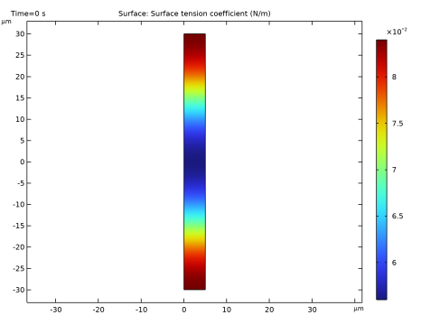
Locate the Surface Tension section. Select the Include surface tension force in momentum equation checkbox.
6
From the Surface tension coefficient list, choose User defined. In the σ text field, type sigma.
Laminar Flow (spf)
In the Model Builder window, under Component 1 (comp1) click Laminar Flow (spf).
Pressure Point Constraint 1
1
In the Physics toolbar, click  Points and choose Pressure Point Constraint.
2
Level Set (ls)
Initial Values, Fluid 2
1
In the Model Builder window, under Component 1 (comp1) > Level Set (ls) click Initial Values, Fluid 2.
2
Laminar Flow (spf)
In the Model Builder window, under Component 1 (comp1) click Laminar Flow (spf).
Symmetry 1
1
In the Physics toolbar, click  Boundaries and choose Symmetry.
2
Level Set (ls)
1
In the Model Builder window, under Component 1 (comp1) click Level Set (ls).
2
In the Physics toolbar, click  Boundaries and choose Symmetry.
Select Boundaries 2, 3, 5, and 6 only.
Mesh 1
Free Triangular 1
In the Mesh toolbar, click  Free Triangular.
Size
1
In the Model Builder window, click Size.
2
In the Settings window for Size, locate the Element Size section.
3
From the Calibrate for list, choose Fluid dynamics.
4
In the Model Builder window, right-click Mesh 1 and choose Build All.
Study 1
Step 2: Time Dependent
1
In the Model Builder window, under Study 1 click Step 2: Time Dependent.
2
In the Settings window for Time Dependent, locate the Study Settings section.
3
In the Output times text field, type range(0,2e-7,2e-5).
4
In the Study toolbar, click  Compute.
Results
2D Plot Group 6
1
In the Results toolbar, click  2D Plot Group.
2
In the Settings window for 2D Plot Group, locate the Plot Settings section.
3
Clear the Plot dataset edges checkbox.
Contour 1
1
Right-click 2D Plot Group 6 and choose Contour.
2
In the Settings window for Contour, locate the Expression section.
3
In the Expression text field, type ls.Vf1.
4
Locate the Levels section. From the Entry method list, choose Levels.
5
In the Levels text field, type 0.5.
6
Locate the Coloring and Style section. From the Contour type list, choose Filled.
7
From the Color table list, choose GrayScale.
8
From the Color table transformation list, choose Reverse.
9
Click the  Zoom Extents button in the Graphics toolbar.
10
In the 2D Plot Group 6 toolbar, click  Plot.
Compare the results with those in Figure 2 at different time steps.
 

1
This model is courtesy of Prof. E. Furlani, Depts. of Chemical/Biological & Electrical Engineering, SUNY Buffalo, USA (formerly at Eastman Kodak, Rochester, NY, USA).