PDF

Using the 3-Omega Method
to Estimate the Thermal Conductivity
of Nanostructured Materials
Introduction
The 3ω method is an experimental technique to estimate the thermal conductivity of nanostructured material samples. The method takes advantage of lock-in amplifier technology and moves the measurement into the frequency domain; the amplitude and the resistance phase variations of the metal wire or strip heater are measured as a function of the excitation frequency (Ref. 1).
In this method a single metal strip is deposited on the surface of specimen. This metal strip is used simultaneously as a heater and a resistance thermometer. The thermal contact between the heater and the specimen is assumed to be ideal. The heat capacity of metal strip is neglected, i.e., the heater is assumed to be an infinitely good thermal conductor. The simplified geometry of the sample with the metal strip is shown in Figure 1.
Figure 1: The simplified geometry of the experimental setup.
The alternating current at frequency ω
passing through the metal strip provides a periodic heat source oscillating at frequency 2ω:
.
This heat source results in oscillations of the space-averaged temperature of the heater at frequency 2ω:
where ΔTmax is an oscillation amplitude and φ is a phase shift.
For small temperature changes the resistance of the heater can be defined as a linear function of temperature:
where β is the temperature coefficient of resistance, R0 and R are the resistances of the metal heater at temperatures T0 and T0 + ΔT, respectively.
The voltage across the heater is calculated by multiplying the heater resistance with the input current. Under the given alternating current, the voltage across the heater has the ω and 3ω components with phase shift, which is the result of multiplying the resistance, oscillating at the frequency 2ω, with the input current, oscillating at the frequency ω. By measuring the frequency dependence of third harmonic (3ω) of voltage it is possible to obtain the information about the thermal conductivity of the sample being tested.
To derive the equation relating the thermal conductivity to the voltage oscillation amplitude for the narrow metal strip heater, we can use the exact solution for the temperature oscillations amplitude in a semi-infinite solid with a line heat source, that can be written approximately as a log-linear function
where ΔTmax is the amplitude of spatially averaged temperature oscillation in the strip, k is the thermal conductivity, and L is the length of the strip. This approximation applies, if the width of the heater strip, w, is much smaller than the thermal penetration depth, δP. The thermal penetration depth is the depth in which heat diffuses during one cycle of the oscillating heat power. At a distance greater than δP the amplitude of the temperature fluctuation is reduced by approximately 90% relative to that of the heater.
The third harmonic (3ω) of voltage has a linear dependence of the temperature amplitude
where V0 is the first harmonic (ω) voltage amplitude.
Thus, if the thermal penetration depth is much larger than the width of the heater strip, the derivative
is constant, and we can calculate the thermal conductivity using the results obtained at two different oscillation frequencies ω1 and ω2:
.
To be sure that the chosen frequencies correspond to the log-linear approximation range, we sweep through a wide range of frequencies to find out the log-linear region for the given conditions.
Model Definition
This COMSOL Multiphysics model solves the coupled electromagnetic heating problem in a solid sample that is heated by a thin copper strip deposited on the surface of the sample, as shown in Figure 2. Since the geometry is symmetrical, only one half of the section is modeled.
Figure 2: The model geometry.
The metal strip has a length L = 5 mm, a width w = 0.1 mm and a thickness th = 0.3 nm. The sample has the same length, the width is equal to 10w, and depth d = 0.3 mm. The geometry is partitioned into several domains. The “infinite domains” (shown in blue color) are used to model the semi-infinite solid. These special domains allow us to truncate the geometry to consider the region near the heater only. We can assign them as Infinite Element Domains and thus suppress boundary effects. The width of Infinite Element Domains is equal to w/2. The model is symmetrical, so we use infinite domains to model the semi-infinite space only on the right and lower boundaries.
The amplitude of third harmonic of the voltage across the heater is evaluated at different frequencies. Analyzing the frequency dependence of the voltage oscillation amplitude, we can determine the log-linear region. We then use this to evaluate the thermal conductivity of a sample and compare the result with the value that is used in the simulation.
Results and Discussion
Figure 3 shows the frequency dependence of the third harmonic of the voltage oscillation amplitude obtained with the time-dependent study. The log-linear region for the given conditions lies in the frequency range from 105 to 10 Hz, as can be seen from the plot.
Figure 3: The frequency dependence of the third harmonic of voltage.
To obtain the thermal conductivity we need to take two points from the log-linear region of the curve and substitute the values into the expression
.
We use the two frequency values f1 = 104 Hz and f2 = 1 Hz and enter them in the Parameters node of the Results section of the model tree. Then we run an evaluation of the thermal conductivity in the Thermal Conductivity Evaluation node. The computed values are displayed in the corresponding table. The estimated value of 1.1181 W/(m·K) is very close to the exact value of 1.11 W/(m·K), that was used in the simulation.
Reference
1. D.G. Cahill, and R.O. Pohl, “Thermal conductivity of amorphous solids above the plateau,” Phys. Rev. B, vol. 35, no. 8, pp. 4067–4073, 1987.
Application Library path: Heat_Transfer_Module/Thermal_Processing/three_omega_method_for_estimating_thermal_conductivity
Modeling Instructions
From the File menu, choose New.
New
In the New window, click  Model Wizard.
Model Wizard
1
In the Model Wizard window, click  3D.
2
In the Select Physics tree, select Heat Transfer > Electromagnetic Heating > Joule Heating.
3
Click Add.
4
Click  Study.
5
In the Select Study tree, select General Studies > Time Dependent.
6
Global Definitions
Parameters 1
1
In the Model Builder window, under Global Definitions click Parameters 1.
2
In the Settings window for Parameters, locate the Parameters section.
3
Geometry 1
Block 1 (blk1)
1
In the Geometry toolbar, click  Block.
2
In the Settings window for Block, locate the Size and Shape section.
3
In the Width text field, type w/2.
4
In the Depth text field, type L.
5
In the Height text field, type th.
Block 2 (blk2)
1
In the Geometry toolbar, click  Block.
2
In the Settings window for Block, locate the Size and Shape section.
3
In the Width text field, type 3*w.
4
In the Depth text field, type L.
5
In the Height text field, type d.
6
Locate the Position section. In the z text field, type -d.
7
Click to expand the Layers section. In the table, enter the following settings:
8
Find the Layer position subsection. Select the Right checkbox.
Form Union (fin)
In the Geometry toolbar, click  Build All.
Definitions
Average 1 (aveop1)
1
In the Definitions toolbar, click  Nonlocal Couplings and choose Average.
2
In the Settings window for Average, locate the Source Selection section.
3
From the Geometric entity level list, choose Boundary.
4
Infinite Element Domain 1 (ie1)
1
In the Definitions toolbar, click  Infinite Element Domain.
2
Ambient Properties 1 (ampr1)
1
In the Physics toolbar, click  Shared Properties and choose Ambient Properties.
2
In the Settings window for Ambient Properties, locate the Ambient Conditions section.
3
In the Tamb text field, type T_ref.
Electric Currents (ec)
1
In the Model Builder window, collapse the Component 1 (comp1) > Electric Currents (ec) node.
2
In the Model Builder window, click Electric Currents (ec).
3
In the Settings window for Electric Currents, locate the Domain Selection section.
4
Click  Clear Selection.
5
Current Conservation 1
1
In the Model Builder window, expand the Electric Currents (ec) node, then click Current Conservation 1.
2
In the Settings window for Current Conservation, locate the Constitutive Relation Jc-E section.
3
From the Conduction model list, choose Linearized resistivity.
Ground 1
1
In the Physics toolbar, click  Boundaries and choose Ground.
2
Normal Current Density 1
1
In the Physics toolbar, click  Boundaries and choose Normal Current Density.
2
3
In the Settings window for Normal Current Density, locate the Normal Current Density section.
4
In the Jn text field, type J0*cos(omega*t).
Symmetry Plane 1
1
In the Physics toolbar, click  Boundaries and choose Symmetry Plane.
2
Heat Transfer in Solids (ht)
Initial Values 1
1
In the Model Builder window, under Component 1 (comp1) > Heat Transfer in Solids (ht) click Initial Values 1.
2
In the Settings window for Initial Values, locate the Initial Values section.
3
From the T list, choose Ambient temperature (ampr1).
Heat Source 1
1
In the Physics toolbar, click  Domains and choose Heat Source.
2
3
In the Settings window for Heat Source, locate the Heat Source section.
4
From the Heat source list, choose Heat rate.
5
In the P0 text field, type -Prms/2.
Temperature 1
1
In the Physics toolbar, click  Boundaries and choose Temperature.
2
3
In the Settings window for Temperature, locate the Temperature section.
4
From the T0 list, choose Ambient temperature (ampr1).
Symmetry 1
1
In the Physics toolbar, click  Boundaries and choose Symmetry.
2
Materials
Sample
1
In the Model Builder window, under Component 1 (comp1) right-click Materials and choose Blank Material.
2
In the Settings window for Material, type Sample in the Label text field.
3
4
Locate the Material Contents section. In the table, enter the following settings:
Add Material
1
In the Materials toolbar, click  Add Material to open the Add Material window.
2
Go to the Add Material window.
3
In the tree, select Built-in > Copper.
4
Click the Add to Component button in the window toolbar.
5
In the Materials toolbar, click  Add Material to close the Add Material window.
Materials
Copper (mat2)
1
2
In the Settings window for Material, locate the Material Contents section.
3
Ω·m
Mesh 1
Mapped 1
1
In the Model Builder window, expand the Component 1 (comp1) > Mesh 1 node.
2
Right-click Mesh 1 and choose More Generators > Mapped.
3
Distribution 1
1
Right-click Mapped 1 and choose Distribution.
2
3
In the Settings window for Distribution, locate the Distribution section.
4
In the Number of elements text field, type 3.
Distribution 2
1
In the Model Builder window, right-click Mapped 1 and choose Distribution.
2
3
In the Settings window for Distribution, locate the Distribution section.
4
In the Number of elements text field, type 10.
Swept 1
In the Mesh toolbar, click  Swept.
Distribution 1
1
Right-click Swept 1 and choose Distribution.
2
In the Settings window for Distribution, locate the Domain Selection section.
3
Click  Clear Selection.
4
5
Locate the Distribution section. In the Number of elements text field, type 2.
Distribution 2
1
In the Model Builder window, right-click Swept 1 and choose Distribution.
2
In the Settings window for Distribution, locate the Domain Selection section.
3
Click  Clear Selection.
4
5
Locate the Distribution section. From the Distribution type list, choose Predefined.
6
In the Number of elements text field, type 10.
7
In the Element ratio text field, type 10.
8
From the Growth rate list, choose Exponential.
Distribution 3
1
Right-click Swept 1 and choose Distribution.
2
In the Settings window for Distribution, locate the Domain Selection section.
3
Click  Clear Selection.
4
5
Locate the Distribution section. In the Number of elements text field, type 3.
6
Click  Build All.
Study 1
Parametric Sweep
1
In the Study toolbar, click  Parametric Sweep.
2
In the Settings window for Parametric Sweep, locate the Study Settings section.
3
4
Step 1: Time Dependent
1
In the Model Builder window, click Step 1: Time Dependent.
2
In the Settings window for Time Dependent, locate the Study Settings section.
3
In the Output times text field, type range(0,0.03,N)/f.
Step 2: Time to Frequency FFT
1
In the Study toolbar, click  Study Steps and choose Frequency Domain > Time to Frequency FFT.
2
In the Settings window for Time to Frequency FFT, locate the Study Settings section.
3
In the Start time text field, type 2/f.
4
In the End time text field, type N/f.
5
In the Maximum output frequency text field, type 5*f.
Solution 1 (sol1)
1
In the Study toolbar, click  Show Default Solver.
2
In the Model Builder window, expand the Solution 1 (sol1) node, then click Time-Dependent Solver 1.
3
In the Settings window for Time-Dependent Solver, click to expand the Time Stepping section.
4
From the Steps taken by solver list, choose Strict.
5
Right-click Study 1 > Solver Configurations > Solution 1 (sol1) > Time-Dependent Solver 1 and choose Fully Coupled.
6
In the Study toolbar, click  Compute.
Results
Voltage Amplitude vs Current Frequency
1
In the Results toolbar, click  Evaluation Group.
2
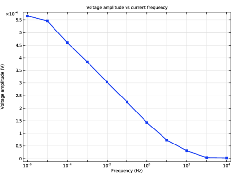
In the Settings window for Evaluation Group, type Voltage Amplitude vs Current Frequency in the Label text field.
Global Evaluation Sweep 1
1
In the Voltage Amplitude vs Current Frequency toolbar, click  More Evaluations and choose Global Evaluation Sweep.
2
In the Settings window for Global Evaluation Sweep, locate the Parameters section.
3
4
Locate the Expressions section. In the table, enter the following settings:
5
In the Voltage Amplitude vs Current Frequency toolbar, click  Evaluate.
Voltage Amplitude vs Current Frequency
1
Go to the Voltage Amplitude vs Current Frequency window.
2
Click the Table Graph button in the window toolbar.
Results
Voltage Amplitude vs Current Frequency
1
In the Model Builder window, under Results click 1D Plot Group 4.
2
In the Settings window for 1D Plot Group, type Voltage Amplitude vs Current Frequency in the Label text field.
3
Locate the Axis section. Select the x-axis log scale checkbox.
4
Locate the Plot Settings section.
5
Select the x-axis label checkbox. In the associated text field, type Frequency (Hz).
6
Select the y-axis label checkbox. In the associated text field, type Voltage amplitude (V).
7
Click to expand the Title section. From the Title type list, choose Manual.
8
In the Title text area, type Voltage amplitude vs current frequency.
Table Graph 1
1
In the Model Builder window, click Table Graph 1.
2
In the Settings window for Table Graph, locate the Coloring and Style section.
3
From the Width list, choose 2.
4
Find the Line markers subsection. From the Marker list, choose Point.
5
In the Voltage Amplitude vs Current Frequency toolbar, click  Plot.
Parameters
1
In the Results toolbar, click  Parameters.
2
In the Settings window for Parameters, locate the Parameters section.
3
Thermal Conductivity Evaluation
1
In the Results toolbar, click  Evaluation Group.
2
In the Settings window for Evaluation Group, type Thermal Conductivity Evaluation in the Label text field.
3
Locate the Data section. From the Parameter selection (freq) list, choose Last.
4
Click to expand the Format section. From the Include parameters list, choose Off.
5
Locate the Transformation section. Select the Transpose checkbox.
Global Evaluation 1
1
Right-click Thermal Conductivity Evaluation and choose Global Evaluation.
2
In the Settings window for Global Evaluation, locate the Expressions section.
3
3ω method
4
In the Thermal Conductivity Evaluation toolbar, click  Evaluate.