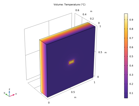
PDF

Thermal Bridges in Building Construction — 3D Iron Bar Through Insulation Layer
Introduction
The European standard EN ISO 10211:2017 for thermal bridges in building constructions provides four test cases — two 2D and two 3D — for validating a numerical method (Ref. 1). If the values obtained by a method conform to the results of all these four cases, the method is classified as a three-dimensional steady-state high precision method.
COMSOL Multiphysics successfully passes all the test cases described by the standard. This document presents an implementation of the second 3D model (Case 4).
This tutorial studies the heat conduction in a thermal bridge made up of an iron bar and an insulation layer that separates a hot internal side from a cold external side. The iron bar is embedded in the insulation layer as shown in Figure 1. After solving the model, the heat flux between the internal and external sides and the maximum temperature on the external wall are calculated, and the results are compared to the expected values.
Figure 1: Back side (left) and front side (right) views of the iron bar embedded in an insulation layer, ISO 10211:2017 test case 4. Colored regions correspond to internal and external boundaries.
Model Definition
The geometry is illustrated above in Figure 1. The square insulation layer, with a low thermal conductivity k of 0.1 W/(m·K), has a cold and a hot surface. The iron bar has a higher thermal conductivity, 50  W/(m·K). Its boundaries are mainly located in the hot environment but one of them reaches the cold side.
Cold and hot surfaces are subject to convective heat flux. The ISO 10211:2017 standard specifies the values of the thermal resistance, R, which is related to the heat transfer coefficient, h, according to
Notes About the COMSOL Implementation
Compared to the rest of the structure, the dimensions of the intersection between the iron bar and the insulation layer are relatively small but the temperature gradients are large. Therefore, the element size is reduced in this area to give sufficient accuracy. To save computational time, this refinement is not applied on the remaining mesh.
Results and Discussion
In Figure 2, the temperature profile shows the effects of the thermal bridge where the heat variations are most pronounced.
Figure 2: Temperature distribution of ISO 10211:2017 test case 4.
Table 1 compares the numerical results of COMSOL Multiphysics with the expected values provided by EN ISO 10211:2017 (Ref. 1).
3.8·10-3°C
The maximum permissible differences to pass this test case are 5·10-3°C for temperature and 1% for heat flux. The measured values are completely coherent and meet the validation criteria.
Reference
1. European Committee for Standardization, EN ISO 10211, Thermal bridges in building construction – Heat flows and surface temperatures – Detailed calculations (ISO 10211:2017), Appendix A, pp. 54–60, 2017.
Application Library path: Heat_Transfer_Module/Buildings_and_Constructions/thermal_bridge_3d_iron_bar
Modeling Instructions
From the File menu, choose New.
New
In the New window, click  Model Wizard.
Model Wizard
1
In the Model Wizard window, click  3D.
2
In the Select Physics tree, select Heat Transfer > Heat Transfer in Solids (ht).
3
Click Add.
4
Click  Study.
5
In the Select Study tree, select General Studies > Stationary.
6
Global Definitions
Define the geometrical parameters.
Parameters 1
1
In the Model Builder window, under Global Definitions click Parameters 1.
2
In the Settings window for Parameters, locate the Parameters section.
3
Geometry 1
Block 1 (blk1)
1
In the Geometry toolbar, click  Block.
2
In the Settings window for Block, locate the Size and Shape section.
3
In the Width text field, type w1.
4
In the Depth text field, type d1.
5
In the Height text field, type h1.
6
Click  Build Selected.
Create the iron bar at the center of the insulation layer.
Block 2 (blk2)
1
In the Geometry toolbar, click  Block.
2
In the Settings window for Block, locate the Size and Shape section.
3
In the Width text field, type w2.
4
In the Depth text field, type d2.
5
In the Height text field, type h2.
6
Locate the Position section. In the x text field, type w1/2-w2/2.
7
In the z text field, type h1/2-h2/2.
8
Click  Build Selected.
9
Click the  Wireframe Rendering button in the Graphics toolbar to get a better view of the interior parts.
To remove the unnecessary interior boundary in the iron bar, proceed as follows.
Ignore Faces 1 (igf1)
1
In the Geometry toolbar, click  Virtual Operations and choose Ignore Faces.
2
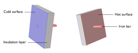
On the object fin, select Boundary 11 only.
Note that you can create the selection by clicking the Paste Selection button and typing the indices in the dialog that opens.
3
In the Geometry toolbar, click  Build All.
4
Click the  Zoom Extents button in the Graphics toolbar.
Definitions
Create a set of selections for use when setting up the physics. First, select the boundaries inside the region y0.1.
Internal
1
In the Definitions toolbar, click  Box.
2
In the Settings window for Box, type Internal in the Label text field.
3
Locate the Geometric Entity Level section. From the Level list, choose Boundary.
4
Locate the Box Limits section. In the y minimum text field, type 0.1.
5
Locate the Output Entities section. From the Include entity if list, choose Entity inside box.
Next, select all the boundaries inside the region y 0.1.
External
1
In the Definitions toolbar, click  Box.
2
In the Settings window for Box, type External in the Label text field.
3
Locate the Geometric Entity Level section. From the Level list, choose Boundary.
4
Locate the Box Limits section. In the y maximum text field, type 0.1.
5
Locate the Output Entities section. From the Include entity if list, choose Entity inside box.
6
Click the  Wireframe Rendering button in the Graphics toolbar.
Materials
Insulation
1
In the Materials toolbar, click  Blank Material.
2
In the Settings window for Material, type Insulation in the Label text field.
3
4
Locate the Material Contents section. In the table, enter the following settings:
Iron
1
In the Materials toolbar, click  Blank Material.
2
In the Settings window for Material, type Iron in the Label text field.
3
4
Locate the Material Contents section. In the table, enter the following settings:
Heat Transfer in Solids (ht)
Heat Flux 1
1
In the Physics toolbar, click  Boundaries and choose Heat Flux.
2
In the Settings window for Heat Flux, locate the Boundary Selection section.
3
From the Selection list, choose Internal.
4
Locate the Heat Flux section. From the Flux type list, choose Convective heat flux.
5
In the h text field, type 1[W/(m^2*K)]/0.10.
6
In the Text text field, type 1[degC].
Heat Flux 2
1
In the Physics toolbar, click  Boundaries and choose Heat Flux.
2
In the Settings window for Heat Flux, locate the Boundary Selection section.
3
From the Selection list, choose External.
4
Locate the Heat Flux section. From the Flux type list, choose Convective heat flux.
5
In the h text field, type 1[W/(m^2*K)]/0.10.
6
In the Text text field, type 0[degC].
Mesh 1
Because the largest temperature variations are expected at the exterior boundary of the iron bar, refine the mesh in this region. Use the default settings in the remaining domains.
Free Tetrahedral 1
In the Mesh toolbar, click  Free Tetrahedral.
Size 1
1
In the Mesh toolbar, click Size Attribute and choose Extremely Fine.
2
In the Settings window for Size, locate the Geometric Entity Selection section.
3
From the Geometric entity level list, choose Domain.
4
5
Click  Build All.
Study 1
In the Study toolbar, click  Compute.
Results
Change the unit of the temperature results to degrees Celsius.
Preferred Units 1
1
In the Results toolbar, click  Configurations and choose Preferred Units.
2
In the Settings window for Preferred Units, locate the Units section.
3
Click  Add Physical Quantity.
4
In the Physical Quantity dialog, select General > Temperature (K) in the tree.
5
6
In the Settings window for Preferred Units, locate the Units section.
7
8
Click  Apply.
The default plot group shows the temperature distribution; compare with Figure 2.
Follow the steps below to calculate the maximum temperature on the external surface and the heat flux between the internal and external sides. Compare the values with the expected results listed in Table 1.
Surface Maximum 1
1
In the Results toolbar, click  More Derived Values and choose Maximum > Surface Maximum.
2
In the Settings window for Surface Maximum, locate the Selection section.
3
From the Selection list, choose External.
4
Click  Evaluate.
Table 1
1
Go to the Table 1 window.
The displayed value should be close to 0.805°C.
Results
Surface Integration 1
1
In the Results toolbar, click  More Derived Values and choose Integration > Surface Integration.
2
In the Settings window for Surface Integration, locate the Selection section.
3
From the Selection list, choose External.
4
Click Replace Expression in the upper-right corner of the Expressions section. From the menu, choose Component 1 (comp1) > Heat Transfer in Solids > Boundary fluxes > ht.q0 - Inward heat flux - W/m².
5
Click  Evaluate.
Table 2
1
Go to the Table 2 window.
The measured flux should be close to 0.540 W.