|
|
|

|
•
|
Primary Current Distribution for modeling the electrolyte potential, governed by Ohm’s Law (Equation 3). The secondary and tertiary current distributions are modeled by changing the current distribution type of the interface to Secondary.
|
|
1
|
|
2
|
In the Select Physics tree, select Electrochemistry > Primary and Secondary Current Distribution > Primary Current Distribution (cd).
|
|
3
|
Click Add.
|
|
4
|
Click
|
|
5
|
|
6
|
Click
|
|
1
|
|
2
|
Browse to the model’s Application Libraries folder and double-click the file wire_electrode_geom_sequence.mph.
|
|
3
|
|
1
|
|
2
|
|
1
|
|
2
|
Go to the Add Material window.
|
|
3
|
|
4
|
Click the Add to Component button in the window toolbar.
|
|
5
|
|
1
|
|
3
|
|
1
|
|
3
|
|
4
|
Click
|
|
5
|
|
6
|
Click OK.
|
|
1
|
|
2
|
|
3
|
|
1
|
|
3
|
|
4
|
Click
|
|
5
|
|
6
|
Click OK.
|
|
7
|
In the Settings window for Electrode Surface, locate the Electrode Phase Potential Condition section.
|
|
8
|
|
1
|
|
2
|
|
3
|
|
1
|
In the Model Builder window, under Component 1 (comp1) > Primary Current Distribution (cd) click Initial Values 1.
|
|
2
|
|
3
|
|
1
|
|
2
|
In the Settings window for Boundary Layer Properties, locate the Geometric Entity Selection section.
|
|
3
|
|
4
|
|
5
|
|
6
|
|
7
|
|
1
|
|
2
|
|
3
|
|
4
|
|
5
|
|
6
|
|
1
|
|
2
|
|
3
|
|
1
|
|
2
|
|
3
|
|
4
|
|
1
|
|
2
|
|
3
|
|
4
|
|
1
|
|
2
|
|
3
|
Select the Auxiliary sweep checkbox.
|
|
4
|
Click
|
|
6
|
|
7
|
|
8
|
Clear the Generate default plots checkbox.
|
|
9
|
|
1
|
|
2
|
|
1
|
In the Model Builder window, under Study 1 > Solver Configurations click Solution 1 - Copy 1 (sol2).
|
|
2
|
|
1
|
|
2
|
|
3
|
|
4
|
|
5
|
Locate the Plot Settings section.
|
|
6
|
|
7
|
|
8
|
|
1
|
|
2
|
|
3
|
|
4
|
Locate the y-Axis Data section. In the table, enter the following settings:
|
|
5
|
|
7
|
|
1
|
|
2
|
|
3
|
|
4
|
|
5
|
|
1
|
|
2
|
|
3
|
|
4
|
|
5
|
|
6
|
|
1
|
|
2
|
|
3
|
|
4
|
|
5
|
|
6
|
Click OK.
|
|
7
|
|
1
|
|
2
|
|
1
|
|
2
|
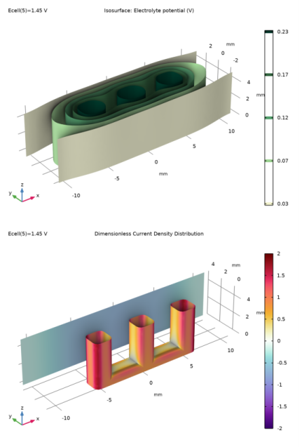
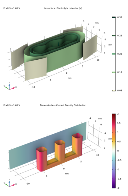
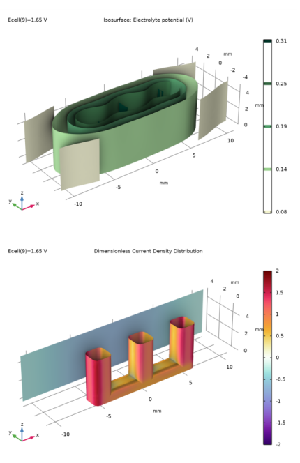
In the Settings window for 3D Plot Group, type Dimensionless Current Density Distribution in the Label text field.
|
|
3
|
|
4
|
|
5
|
|
6
|
|
7
|
|
8
|
|
1
|
|
2
|
|
3
|
|
4
|
|
5
|
|
6
|
|
7
|
|
8
|
|
9
|
|
1
|
|
2
|
In the Settings window for Primary Current Distribution, locate the Current Distribution Type section.
|
|
3
|
|
1
|
|
2
|
|
1
|
In the Model Builder window, under Component 1 (comp1) > Secondary Current Distribution (cd) > Electrode Surface 1 click Electrode Reaction 1.
|
|
2
|
|
3
|
|
4
|
|
5
|
|
6
|
|
1
|
In the Model Builder window, under Component 1 (comp1) > Secondary Current Distribution (cd) > Electrode Surface 2 click Electrode Reaction 1.
|
|
2
|
|
3
|
|
4
|
|
5
|
|
6
|
|
1
|
|
2
|
|
3
|
|
4
|
|
1
|
|
2
|
|
1
|
In the Model Builder window, under Results > Polarization Plot right-click Global 1 and choose Duplicate.
|
|
2
|
|
3
|
|
4
|
Locate the Legends section. In the table, enter the following settings:
|
|
1
|
|
2
|
|
1
|
|
2
|
|
3
|
|
4
|
|
5
|
|
6
|
|
1
|
|
2
|
|
3
|
|
4
|
|
5
|
|
6
|
|
1
|
|
2
|
|
1
|
|
2
|
Go to the Add Physics window.
|
|
3
|
|
4
|
Click the Add to Component 1 button in the window toolbar.
|
|
5
|
|
6
|
Click the Add to Component 1 button in the window toolbar.
|
|
7
|
|
1
|
|
2
|
Select the Migration in electric field checkbox.
|
|
1
|
In the Model Builder window, under Component 1 (comp1) > Transport of Diluted Species (tds) click Species Charges.
|
|
2
|
|
3
|
|
1
|
|
2
|
|
3
|
|
1
|
|
3
|
|
4
|
Click
|
|
5
|
|
6
|
Click OK.
|
|
7
|
|
8
|
|
1
|
|
3
|
|
4
|
Click
|
|
5
|
|
6
|
Click OK.
|
|
1
|
|
2
|
|
3
|
|
1
|
|
2
|
|
3
|
|
1
|
In the Model Builder window, expand the Electrode Surface Coupling 1 node, then click Reaction Coefficients 1.
|
|
2
|
|
3
|
|
4
|
|
1
|
In the Model Builder window, under Component 1 (comp1) > Secondary Current Distribution (cd) > Electrode Surface 2 click Electrode Reaction 1.
|
|
2
|
|
3
|
|
4
|
|
5
|
|
6
|
Locate the Electrode Kinetics section. From the Exchange current density type list, choose From Nernst Equation.
|
|
7
|
|
1
|
|
2
|
|
3
|
|
4
|
|
5
|
|
1
|
|
2
|
|
3
|
|
4
|
|
1
|
|
3
|
|
4
|
|
1
|
|
1
|
|
2
|
Go to the Add Study window.
|
|
3
|
|
4
|
Click the Add Study button in the window toolbar.
|
|
5
|
|
1
|
|
2
|
In the Solve for column of the table, under Component 1 (comp1), clear the checkboxes for Secondary Current Distribution (cd) and Transport of Diluted Species (tds).
|
|
1
|
|
2
|
|
3
|
In the Solve for column of the table, under Component 1 (comp1), clear the checkbox for Laminar Flow (spf).
|
|
4
|
|
5
|
Click
|
|
1
|
|
2
|
|
3
|
In the Model Builder window, expand the Study 2 > Solver Configurations > Solution 3 (sol3) > Stationary Solver 2 node.
|
|
4
|
Right-click Study 2 > Solver Configurations > Solution 3 (sol3) > Stationary Solver 2 and choose Fully Coupled.
|
|
5
|
|
6
|
|
7
|
|
8
|
|
9
|
Clear the Generate default plots checkbox.
|
|
10
|
|
11
|
|
1
|
In the Model Builder window, under Results > Polarization Plot right-click Global 2 and choose Duplicate.
|
|
2
|
|
3
|
|
4
|
Locate the Legends section. In the table, enter the following settings:
|
|
5
|
|
1
|
|
2
|
|
3
|
Locate the Data section. From the Dataset list, choose Tertiary Current Distribution/Solution 3 (sol3).
|
|
1
|
|
2
|
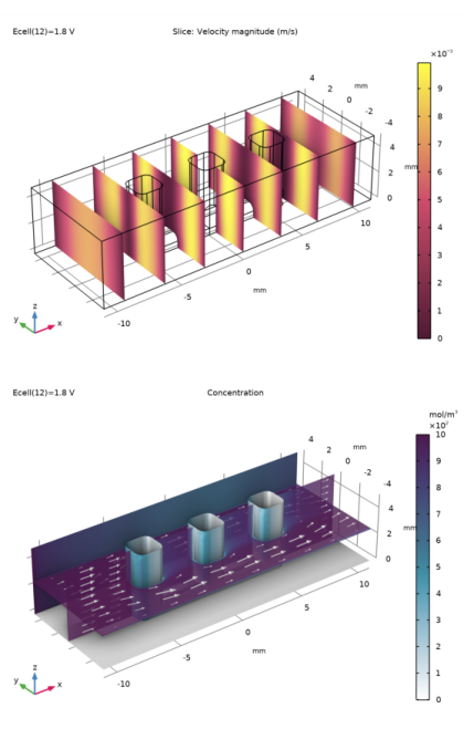
In the Settings window for Slice, click Replace Expression in the upper-right corner of the Expression section. From the menu, choose Component 1 (comp1) > Laminar Flow > Velocity and pressure > spf.U - Velocity magnitude - m/s.
|
|
3
|
|
4
|
|
5
|
|
6
|
|
7
|
|
1
|
|
2
|
|
3
|
Locate the Data section. From the Dataset list, choose Tertiary Current Distribution/Solution 3 (sol3).
|
|
4
|
|
5
|
|
6
|
|
1
|
|
2
|
In the Settings window for Arrow Volume, click Replace Expression in the upper-right corner of the Expression section. From the menu, choose Component 1 (comp1) > Laminar Flow > Velocity and pressure > u,v,w - Velocity field.
|
|
3
|
Locate the Arrow Positioning section. Find the x grid points subsection. In the Points text field, type 10.
|
|
4
|
|
5
|
|
6
|
|
1
|
|
2
|
|
3
|
|
4
|
Locate the Arrow Positioning section. Find the y grid points subsection. In the Points text field, type 1.
|
|
5
|
|
6
|
|
7
|
|
1
|
|
2
|
In the Settings window for Multislice, click Replace Expression in the upper-right corner of the Expression section. From the menu, choose Component 1 (comp1) > Transport of Diluted Species > Species c > c - Molar concentration, c - mol/m³.
|
|
3
|
|
4
|
|
1
|
|
2
|
|
3
|
Clear the Affected by lighting checkbox.
|
|
1
|
|
2
|
|
3
|
|
1
|
|
2
|
|
3
|
Click Replace Expression in the upper-right corner of the Expression section. From the menu, choose Component 1 (comp1) > Transport of Diluted Species > Species c > c - Molar concentration, c - mol/m³.
|
|
4
|
|
1
|
|
2
|
|
3
|
|
1
|
|
2
|
|
1
|
|
2
|
|
3
|
|
1
|
|
1
|
|
2
|
Click Replace Expression in the upper-right corner of the Expression section. From the menu, choose Component 1 (comp1) > Transport of Diluted Species > Species c > c - Molar concentration, c - mol/m³.
|
|
3
|
|
1
|
|
3
|
|
1
|
|
2
|
|
3
|
|
4
|
|
1
|
|
2
|
|
3
|
|
4
|
|
5
|
|
1
|
|
2
|
|
1
|
|
2
|
|
3
|
Select the Wireframe rendering checkbox.
|
|
1
|
|
2
|
|
3
|
|
4
|
|
5
|
|
6
|
|
7
|
|
1
|
|
2
|
|
1
|
|
2
|
|
3
|
|
1
|
|
2
|
|
3
|
|
4
|
|
5
|
|
6
|
Locate the Selections of Resulting Entities section. Select the Resulting objects selection checkbox.
|
|
1
|
|
2
|
On the object sq1, select Points 1–4 only.
|
|
3
|
|
4
|
|
5
|
Locate the Selections of Resulting Entities section. Select the Resulting objects selection checkbox.
|
|
1
|
|
2
|
Select the object fil1 only.
|
|
3
|
|
4
|
|
5
|
|
1
|
In the Model Builder window, expand the Component 1 (comp1) > Geometry 1 > Work Plane 1 (wp1) > View 2 node.
|
|
2
|
|
3
|
|
5
|
Locate the Selections of Resulting Entities section. Find the Cumulative selection subsection. From the Contribute to list, choose Union.
|
|
1
|
|
2
|
|
3
|
|
4
|
|
1
|
|
2
|
|
3
|
|
4
|
|
5
|
Locate the Selections of Resulting Entities section. Select the Resulting objects selection checkbox.
|
|
1
|
|
2
|
On the object sq1, select Points 1–4 only.
|
|
3
|
|
4
|
|
1
|
In the Model Builder window, expand the Component 1 (comp1) > Geometry 1 > Work Plane 2 (wp2) > View 3 node.
|
|
2
|
|
3
|
|
5
|
Select the Reverse direction checkbox.
|
|
6
|
Locate the Selections of Resulting Entities section. Find the Cumulative selection subsection. From the Contribute to list, choose Union.
|
|
1
|
|
2
|
|
3
|
|
1
|
|
2
|
|
3
|
|
4
|
|
5
|
|
6
|
Locate the Selections of Resulting Entities section. Select the Resulting objects selection checkbox.
|
|
1
|
|
2
|
|
3
|
|
1
|
|
2
|
Select the object blk1 only.
|
|
1
|
|
2
|
|
3
|
Select the Resulting objects selection checkbox.
|
|
1
|
|
2
|
|
3
|
|
1
|
|
2
|
|
3
|
|
4
|
|
5
|
|
6
|
|
7
|
|
1
|
|
2
|
|
3
|
|
4
|
Click in the Graphics window and then press Ctrl+D to clear all objects.
|
|
1
|
In the Model Builder window, under Component 1 (comp1) > Geometry 1 click Box Selection 1 (boxsel1).
|
|
2
|
|
3
|
|
1
|
|
2
|
|
3
|
|
4
|
On the object dif1, select Boundaries 2 and 5 only.
|
|
1
|
In the Model Builder window, under Component 1 (comp1) > Geometry 1, Ctrl-click to select Anode (boxsel1) and Cathodes (sel1).
|
|
2
|
Right-click and choose Move Down.
|
|
1
|
|
2
|
|
3
|
|
4
|
|
5
|
On the object fin, select Boundary 1 only.
|
|
1
|
|
2
|
|
3
|
|
4
|
On the object fin, select Boundary 52 only.
|
|
5
|