PDF

Stray Currents from a Train in a Light Rail Transit System
Introduction
Light rail transit (LRT) systems often utilize DC power for train propulsion. In these systems, trains operate with current fed from traction substations (TSS) through overhead lines and the rails usually serve as conductors for the returning current. Since the rails are more or less in contact with the surrounding soil, portions of the returning current can be stray. To avoid corrosion of adjacent metallic structures when building new railways, the stray currents often need to be considered.
This example models stray currents from a moving train in an LRT system and the resulting corrosion of a nearby pipe. The 3D domain surrounding the rails and the pipe features different soil conductivities. The impact of changed soil conductivities and pipe position is also investigated.
Model Definition
The model geometry is shown in Figure 1.
Figure 1: 3D model geometry.
Soil layers, tracks (rails sitting on ties and gravel), and a pipe are accounted for. The soil profile has a radius of 750 m and a depth confined by insulating rock. The pipe is positioned at a depth of 2.5 m. Start and end stations for the train are located near traction substations, denoted “TSS 1” and “TSS 2”, respectively. It takes 90 s for the train to travel between the stations. The distance between the two substations is 1.24 km.
The Cathodic Protection interface is used to solve for the electrolyte potential, ϕl (SI unit: V), over the 3D domains according to:
(1)
where il (SI unit: A/m2) is the electrolyte current density vector and σl (SI unit: S/m) is the electrolyte conductivity for the soil domain. Electrolyte nodes are used at each domain to set different electrolyte conductivities.
The rails and pipe are modeled using Edge Electrode nodes. At each node, the kinetics of the electrochemical reaction is prescribed as:
(2)
where fs,edge − ϕl,edge) is an interpolation function obtained form the experimental polarization data for steel, available in the Corrosion folder in the Material Library.
At the rail edges, the Ohm’s Law electric potential model is defined. At the TSS 2 boundaries, an Electric Potential of 0 V (ground) is set. At the TSS 1 boundaries, an Electrode Current node is used to define the traction substation current-feed to the train. The feed is shared between the two traction substations and depends on train location. Consequently, the current at TSS 1, Itss1, is defined as:
(3)
where the train propulsion current, Itrain, and location, loctrain, are modeled using time-dependent interpolation functions (Figure 2). Lrail is the length of the rail between the two traction substations.
The train propulsion current is defined using an External Current Source node in the Edge Electrode node for the rails. The current source, ql,s, is set up using the Itrain and loctrain function together with a Gaussian Pulse to model the current source where the train is located.
At the pipe edge, the electric potential model is set to floating potential with zero applied current, which indicates that the pipe is electrically not connected to anything and it will interact with the adjacent soil domain only through the electrochemical reactions occurring at the pipe surface.
Results and Discussion
Figure 2 shows the train propulsion current together with the current fed from each TSS with time. The location of the train is included as well and indicates where along the rails the propulsion current is drawn.
Figure 2: Left y-axis: Train propulsion current (Itrain) and computed current feed from TSS 1 and TSS 2. Right x-axis: Train location (loctrain) in terms of traveled distance.
In Figure 3, the potential and pipe current-density distributions are shown for the soil profile when the train has passed more than half of the distance between the stations. Variations in potential are shown across the soil surface. At a distance of about 100 m from the train the potential drops rapidly. Where the pipe is positioned, the potential is nonuniform which explains the currents at the pipe and highlights that stray current from the train corrodes the pipe.
Figure 3: Results at 54 s. Potential distribution in the soil profile with gray arrowed streamlines indicating electrolyte current paths (at the same depth as the pipe). Colored arrows display the current density distribution at the pipe. The straight thick line in gray shows the rails with the black section indicating the location of the train.
Figure 3 displays the potential in one of the rails for different train locations. Note that the train moves solely between x-coordinates 0 to 1200 m and that the modeled rails are slightly longer. The potential gradients constitute the origin of the stray current.
Figure 4: The potential in the upper rail for different times. Square marks the train location.
In Figure 5, the stray current densities show that larger potential gradients in the rail results in larger stray currents. Positive and negative current density values indicate exiting and entering current, respectively.
Figure 5: Stray current density at the upper rail for different times. Square marks the train location.
The current density at the pipe is seen in Figure 6. At 54 s, the train seems to induce the highest corrosion currents (0) at the pipe.
Figure 6: Current density at the pipe at different times.
The corrosion rate of the pipe is affected by the soil conditions and its position. The impact was simulated as well and is shown at 54 s in Figure 7. Repositioning the pipe mitigates corrosion more than changed soil resistivity.
Figure 7: Corrosion rate at pipe at 54 s for three different scenarios.
Notes About the COMSOL Implementation
Since no processes in the model accumulate with time, a Stationary solver using an Auxiliary sweep with time as parameter can be used. This approach reduces the computation time.
References
1. Z. Cai, X. Zhang, and H. Cheng, “Evaluation of DC-Subway Stray Current Corrosion With Integrated Multi-Physical Modeling and Electrochemical Analysis,” IEEE Access, vol. 7, p. 168404, 2019.
2. S. Aatif, H. Hu, F. Rafiq, and Z. He, “Analysis of rail potential and stray current in MVDC railway electrification system,” Railway Engineering Science, vol. 29, p. 394, 2019.
3. G. Du, D. Zhang, G. Li, C. Wang, and J. Liu, “Evaluation of Rail Potential Based on Power Distribution in DC Traction Power Systems,” Energies, vol. 9, p. 729, 2016.
Application Library path: Corrosion_Module/General_Corrosion/stray_current_train
Modeling Instructions
From the File menu, choose New.
New
In the New window, click  Model Wizard.
Model Wizard
1
In the Model Wizard window, click  3D.
2
In the Select Physics tree, select Electrochemistry > Cathodic Protection (cp).
3
Click Add.
4
Click  Study.
5
In the Select Study tree, select General Studies > Stationary.
6
Global Definitions
Load the model parameters from a text file.
Parameters 1
1
In the Model Builder window, under Global Definitions click Parameters 1.
2
In the Settings window for Parameters, locate the Parameters section.
3
Click  Load from File.
4
Use a Gaussian Pulse function to describe the shape of the train positioning at the rails. Set the integrated value to 1 and the standard deviation value to 4 for a simpler and more realistic train representation.
Gaussian Pulse - Shape Train Positioning
1
In the Home toolbar, click  Functions and choose Global > Gaussian Pulse.
2
In the Settings window for Gaussian Pulse, type Gaussian Pulse - Shape Train Positioning in the Label text field.
3
In the Function name text field, type shape_train.
4
Locate the Parameters section. In the Standard deviation text field, type 4.
The train propulsion current with travel time is imported using an Interpolation function.
Interpolation - Train Propulsion Current
1
In the Home toolbar, click  Functions and choose Global > Interpolation.
2
In the Settings window for Interpolation, type Interpolation - Train Propulsion Current in the Label text field.
3
Locate the Definition section. In the Function name text field, type I_train.
4
Click  Load from File.
5
6
Locate the Units section. In the Function table, enter the following settings:
7
In the Argument table, enter the following settings:
The train location with travel time is also imported using an Interpolation function.
Interpolation - Train Location
1
In the Home toolbar, click  Functions and choose Global > Interpolation.
2
In the Settings window for Interpolation, type Interpolation - Train Location in the Label text field.
3
Locate the Definition section. In the Function name text field, type loc_train.
4
Click  Load from File.
5
6
Locate the Units section. In the Function table, enter the following settings:
7
In the Argument table, enter the following settings:
Geometry 1
Import the geometry of the tracks and soil profile from a geometry file.
Import 1 (imp1)
1
In the Geometry toolbar, click  Import.
2
In the Settings window for Import, locate the Source section.
3
Click  Browse.
4
5
Click  Import.
Draw the pipe in the imported geometry. Use parameter L_rePos that easily can be changed to reposition the pipe.
Work Plane - Pipe
1
In the Geometry toolbar, click  Work Plane.
2
In the Settings window for Work Plane, type Work Plane - Pipe in the Label text field.
3
Locate the Plane Definition section. In the z-coordinate text field, type z_pipe.
Work Plane - Pipe (wp1) > Plane Geometry
In the Model Builder window, click Plane Geometry.
Work Plane - Pipe (wp1) > Polygon 1 (pol1)
1
In the Work Plane toolbar, click  Polygon.
2
In the Settings window for Polygon, locate the Object Type section.
3
From the Type list, choose Open curve.
4
Locate the Coordinates section. In the table, enter the following settings:
5
In the Home toolbar, click  Build All.
Disable the analysis of the geometry as the remaining small geometric details are needed.
6
In the Model Builder window, click Geometry 1.
7
In the Settings window for Geometry, locate the Cleanup section.
8
Clear the Automatic detection of small details checkbox.
Definitions
Railway Ties
1
In the Definitions toolbar, click  Explicit.
2
In the Settings window for Explicit, type Railway Ties in the Label text field.
3
Locate the Input Entities section. Click  Paste Selection.
4
In the Paste Selection dialog, type 4,7,9 in the Selection text field.
5
Gravel
1
In the Definitions toolbar, click  Explicit.
2
In the Settings window for Explicit, type Gravel in the Label text field.
3
Locate the Input Entities section. Click  Paste Selection.
4
In the Paste Selection dialog, type 3,6,8 in the Selection text field.
5
Clay
1
In the Definitions toolbar, click  Explicit.
2
In the Settings window for Explicit, type Clay in the Label text field.
3
Locate the Input Entities section. Click  Paste Selection.
4
In the Paste Selection dialog, type 1 in the Selection text field.
5
Pond
1
In the Definitions toolbar, click  Explicit.
2
In the Settings window for Explicit, type Pond in the Label text field.
3
Locate the Input Entities section. Click  Paste Selection.
4
In the Paste Selection dialog, type 2 in the Selection text field.
5
Sandy Clay
1
In the Definitions toolbar, click  Explicit.
2
In the Settings window for Explicit, type Sandy Clay in the Label text field.
3
Locate the Input Entities section. Click  Paste Selection.
4
In the Paste Selection dialog, type 5 in the Selection text field.
5
Pipe
1
In the Definitions toolbar, click  Explicit.
2
In the Settings window for Explicit, type Pipe in the Label text field.
3
Locate the Input Entities section. From the Geometric entity level list, choose Edge.
4
Click  Paste Selection.
5
In the Paste Selection dialog, type 34,55,135 in the Selection text field.
6
Rails
1
In the Definitions toolbar, click  Explicit.
2
In the Settings window for Explicit, type Rails in the Label text field.
3
Locate the Input Entities section. From the Geometric entity level list, choose Edge.
4
Click  Paste Selection.
5
In the Paste Selection dialog, type 30,31,96,98,177,179 in the Selection text field.
6
Upper Rail
1
In the Definitions toolbar, click  Explicit.
2
In the Settings window for Explicit, type Upper Rail in the Label text field.
3
Locate the Input Entities section. From the Geometric entity level list, choose Edge.
4
Click  Paste Selection.
5
In the Paste Selection dialog, type 31,98,179 in the Selection text field.
6
Steel
1
In the Definitions toolbar, click  Explicit.
2
In the Settings window for Explicit, type Steel in the Label text field.
3
Locate the Input Entities section. From the Geometric entity level list, choose Edge.
4
Click  Paste Selection.
5
In the Paste Selection dialog, type 30,31,34,55,96,98,135,177,179 in the Selection text field.
6
TSS 1
1
In the Definitions toolbar, click  Explicit.
2
In the Settings window for Explicit, type TSS 1 in the Label text field.
3
Locate the Input Entities section. From the Geometric entity level list, choose Point.
4
Click  Paste Selection.
5
In the Paste Selection dialog, type 14,15 in the Selection text field.
6
TSS 2
1
In the Definitions toolbar, click  Explicit.
2
In the Settings window for Explicit, type TSS 2 in the Label text field.
3
Locate the Input Entities section. From the Geometric entity level list, choose Point.
4
Click  Paste Selection.
5
In the Paste Selection dialog, type 114,115 in the Selection text field.
6
Add some Integration operators for postprocessing.
Integration - TSS 1
1
In the Definitions toolbar, click  Nonlocal Couplings and choose Integration.
2
In the Settings window for Integration, type Integration - TSS 1 in the Label text field.
3
In the Operator name text field, type intop_tss1.
4
Locate the Source Selection section. From the Geometric entity level list, choose Point.
5
From the Selection list, choose TSS 1.
Integration - TSS 2
1
In the Definitions toolbar, click  Nonlocal Couplings and choose Integration.
2
In the Settings window for Integration, type Integration - TSS 2 in the Label text field.
3
In the Operator name text field, type intop_tss2.
4
Locate the Source Selection section. From the Geometric entity level list, choose Point.
5
From the Selection list, choose TSS 2.
Define a maximum operator at the upper rail to be used for postprocessing.
Maximum - Upper Rail
1
In the Definitions toolbar, click  Nonlocal Couplings and choose Maximum.
2
In the Settings window for Maximum, type Maximum - Upper Rail in the Label text field.
3
In the Operator name text field, type maxop_uprail.
4
Locate the Source Selection section. From the Geometric entity level list, choose Edge.
5
From the Selection list, choose Upper Rail.
Define variables at various locations in the geometry.
Variables - Rails
1
In the Home toolbar, click  Variables and choose Local Variables.
2
In the Settings window for Variables, type Variables - Rails in the Label text field.
3
Locate the Geometric Entity Selection section. From the Geometric entity level list, choose Edge.
4
From the Selection list, choose Rails.
5
Locate the Variables section. In the table, enter the following settings:
Variables - Pipe
1
In the Home toolbar, click  Variables and choose Local Variables.
2
In the Settings window for Variables, type Variables - Pipe in the Label text field.
3
Locate the Geometric Entity Selection section. From the Geometric entity level list, choose Edge.
4
From the Selection list, choose Pipe.
5
Locate the Variables section. In the table, enter the following settings:
Variables - TSS 1
1
In the Home toolbar, click  Variables and choose Local Variables.
2
In the Settings window for Variables, type Variables - TSS 1 in the Label text field.
3
Locate the Geometric Entity Selection section. From the Geometric entity level list, choose Point.
4
From the Selection list, choose TSS 1.
5
Locate the Variables section. In the table, enter the following settings:
Variables - TSS 2
1
In the Home toolbar, click  Variables and choose Local Variables.
2
In the Settings window for Variables, type Variables - TSS 2 in the Label text field.
3
Locate the Geometric Entity Selection section. From the Geometric entity level list, choose Point.
4
From the Selection list, choose TSS 2.
5
Locate the Variables section. In the table, enter the following settings:
Add steel in soil from the Material Library for the metallic objects (rails and pipe).
Add Material
1
In the Materials toolbar, click  Add Material to open the Add Material window.
2
Go to the Add Material window.
3
In the tree, select Corrosion > Iron Alloys (Steels) > Q235 steel in soil.
4
Click the Add to Component button in the window toolbar.
5
In the Materials toolbar, click  Add Material to close the Add Material window.
Set up the physics. Start with the conductivities in each material.
Cathodic Protection (cp)
Electrolyte - Clay
1
In the Settings window for Electrolyte, type Electrolyte - Clay in the Label text field.
2
Locate the Electrolyte section. From the σl list, choose User defined. In the associated text field, type 1/rho_clay.
Electrolyte - Pond
1
In the Physics toolbar, click  Domains and choose Electrolyte.
2
In the Settings window for Electrolyte, type Electrolyte - Pond in the Label text field.
3
Locate the Domain Selection section. From the Selection list, choose Pond.
4
Locate the Electrolyte section. From the σl list, choose User defined. In the associated text field, type 1/rho_pond.
Electrolyte - Sandy Clay
1
In the Physics toolbar, click  Domains and choose Electrolyte.
2
In the Settings window for Electrolyte, type Electrolyte - Sandy Clay in the Label text field.
3
Locate the Domain Selection section. From the Selection list, choose Sandy Clay.
4
Locate the Electrolyte section. From the σl list, choose User defined. In the associated text field, type 1/rho_sand.
Electrolyte - Ties
1
In the Physics toolbar, click  Domains and choose Electrolyte.
2
In the Settings window for Electrolyte, type Electrolyte - Ties in the Label text field.
3
Locate the Domain Selection section. From the Selection list, choose Railway Ties.
4
Locate the Electrolyte section. From the σl list, choose User defined. From the list, choose Diagonal.
Since the ties are discontinuous in the x direction (ties separated by gravel), define an anisotropic conductivity.
5
Specify the σl matrix as
Electrolyte - Gravel
1
In the Physics toolbar, click  Domains and choose Electrolyte.
2
In the Settings window for Electrolyte, type Electrolyte - Gravel in the Label text field.
3
Locate the Domain Selection section. From the Selection list, choose Gravel.
4
Locate the Electrolyte section. From the σl list, choose User defined. In the associated text field, type 1/rho_gravel.
Use the Edge Electrode node to define the rail properties.
Edge Electrode - Rails
1
In the Physics toolbar, click  Edges and choose Edge Electrode.
2
In the Settings window for Edge Electrode, type Edge Electrode - Rails in the Label text field.
3
Locate the Edge Selection section. From the Selection list, choose Rails.
4
Locate the Edge Electrode Properties section. In the redge text field, type r_rail.
The insulation of the rail can be adjusted in the Film Resistance section.
5
Click to expand the Film Resistance section. From the Film resistance list, choose Surface resistance.
6
In the Rfilm text field, type R_railins.
Electrode Reaction 1
Choose the electrode kinetics from the material that was selected earlier.
1
In the Model Builder window, click Electrode Reaction 1.
2
In the Settings window for Electrode Reaction, locate the Equilibrium Potential section.
3
From the Eeq list, choose From material.
4
Locate the Electrode Kinetics section. From the iloc,expr list, choose From material.
The electrode current is set at TSS 1 and ground at TSS 2.
Edge Electrode - Rails
In the Model Builder window, click Edge Electrode - Rails.
Electrode Current - TSS 1
1
In the Physics toolbar, click  Attributes and choose Electrode Current.
2
In the Settings window for Electrode Current, type Electrode Current - TSS 1 in the Label text field.
3
Locate the Point Selection section. From the Selection list, choose TSS 1.
4
Locate the Electrode Current section. In the Is,total text field, type I_tss1.
Edge Electrode - Rails
In the Model Builder window, click Edge Electrode - Rails.
Electric Potential - TSS 2
1
In the Physics toolbar, click  Attributes and choose Electric Potential.
2
In the Settings window for Electric Potential, type Electric Potential - TSS 2 in the Label text field.
3
Locate the Point Selection section. From the Selection list, choose TSS 2.
Use the External Current Source to define the current locally with train location.
Edge Electrode - Rails
In the Model Builder window, click Edge Electrode - Rails.
External Current Source - Train
1
In the Physics toolbar, click  Attributes and choose External Current Source.
2
In the Settings window for External Current Source, type External Current Source - Train in the Label text field.
3
Locate the External Current Source section. In the ql,s text field, type qls_rail.
Add an additional Edge Electrode node and define the conditions at the pipe.
Edge Electrode - Pipe
1
In the Physics toolbar, click  Edges and choose Edge Electrode.
2
In the Settings window for Edge Electrode, type Edge Electrode - Pipe in the Label text field.
3
Locate the Edge Selection section. From the Selection list, choose Pipe.
4
Locate the Edge Electrode Properties section. In the redge text field, type r_pipe.
5
Locate the Electric Potential section. From the Electric potential model list, choose Floating potential.
Electrode Reaction 1
1
In the Model Builder window, click Electrode Reaction 1.
2
In the Settings window for Electrode Reaction, locate the Equilibrium Potential section.
3
From the Eeq list, choose From material.
4
Locate the Electrode Kinetics section. From the iloc,expr list, choose From material.
Add the conductivity of steel in the selected material.
Materials
Q235 steel in soil (mat1)
1
In the Model Builder window, under Component 1 (comp1) > Materials click Q235 steel in soil (mat1).
2
In the Settings window for Material, locate the Geometric Entity Selection section.
3
From the Geometric entity level list, choose Edge.
4
From the Selection list, choose Steel.
5
Locate the Material Contents section. In the table, enter the following settings:
Define a mesh that refines the meshes at and near the rails and pipe.
Mesh 1
1
In the Model Builder window, under Component 1 (comp1) click Mesh 1.
2
In the Settings window for Mesh, locate the Physics-Controlled Mesh section.
3
In the table, clear the Use checkbox for Geometric Analysis, Detail Size.
4
Locate the Sequence Type section. From the list, choose User-controlled mesh.
Size
1
In the Model Builder window, under Component 1 (comp1) > Mesh 1 click Size.
2
In the Settings window for Size, locate the Element Size section.
3
From the Predefined list, choose Coarse.
4
Click  Build All.
Size 1
1
In the Model Builder window, right-click Free Tetrahedral 1 and choose Size.
2
In the Settings window for Size, locate the Geometric Entity Selection section.
3
From the Geometric entity level list, choose Domain.
4
From the Selection list, choose Gravel.
Size 2
1
Right-click Free Tetrahedral 1 and choose Size.
2
In the Settings window for Size, locate the Geometric Entity Selection section.
3
From the Geometric entity level list, choose Edge.
4
From the Selection list, choose Pipe.
5
Locate the Element Size section. Click the Custom button.
6
Locate the Element Size Parameters section.
7
Select the Maximum element size checkbox. In the associated text field, type 10.
Size 3
1
Right-click Free Tetrahedral 1 and choose Size.
2
In the Settings window for Size, locate the Geometric Entity Selection section.
3
From the Geometric entity level list, choose Domain.
4
From the Selection list, choose Railway Ties.
5
Locate the Element Size section. Click the Custom button.
6
Locate the Element Size Parameters section.
7
Select the Maximum element size checkbox. In the associated text field, type 3.
8
Select the Maximum element size checkbox. In the associated text field, type 2.
9
Select the Resolution of narrow regions checkbox. In the associated text field, type 1.
10
Click  Build All.
To investigate different corrosion mitigation approaches add a Parametric sweep. Use the Auxiliary sweep in the Stationary study step to compute the positions of the train during its 90 s journey between the stations.
Study 1
Parametric Sweep
1
In the Study toolbar, click  Parametric Sweep.
2
In the Settings window for Parametric Sweep, locate the Study Settings section.
3
4
5
6
Ω*m
Step 1: Stationary
1
In the Model Builder window, click Step 1: Stationary.
2
In the Settings window for Stationary, click to expand the Study Extensions section.
3
Select the Auxiliary sweep checkbox.
4
5
6
In the Home toolbar, click  Compute.
Results
A few plots are added by default. The following steps shows how the figures in the model documentation are made.
Start with the plot that shows the distributions in current and potential in the soil profile (Figure 3).
Potential and Current Density Distribution (cp)
1
In the Model Builder window, under Results click Electrolyte Current Density (cp).
2
In the Settings window for 3D Plot Group, type Potential and Current Density Distribution (cp) in the Label text field.
3
Locate the Data section. From the Parameter value (t_train (s)) list, choose 54.
4
Click to expand the Title section. From the Title type list, choose Manual.
5
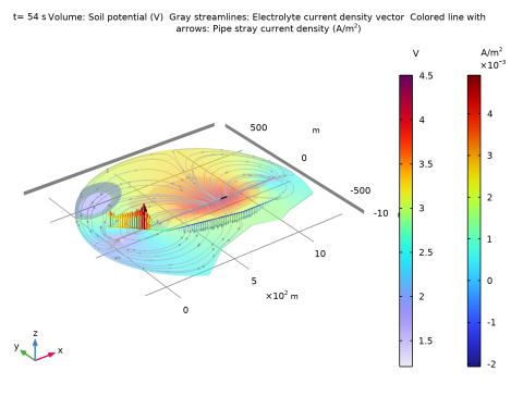
In the Title text area, type Volume: Soil potential (V) Gray streamlines: Electrolyte current density vector Colored line with arrows: Pipe stray current density (A/m<sup>2</sup>).
6
In the Parameter indicator text field, type t= eval(t_train) s.
7
Locate the Plot Settings section. Clear the Plot dataset edges checkbox.
8
Locate the Color Legend section. Select the Show units checkbox.
Volume 1
In the Potential and Current Density Distribution (cp) toolbar, click  Volume.
Streamline 1
In the Model Builder window, right-click Streamline 1 and choose Delete.
Volume - Soil potential
1
In the Settings window for Volume, type Volume - Soil potential in the Label text field.
2
Locate the Coloring and Style section. From the Color table list, choose Prism.
Selection 1
1
In the Potential and Current Density Distribution (cp) toolbar, click  Selection.
2
In the Settings window for Selection, locate the Selection section.
3
From the Selection list, choose Clay.
Volume - Soil potential
In the Model Builder window, click Volume - Soil potential.
Transparency 1
1
In the Potential and Current Density Distribution (cp) toolbar, click  Transparency.
2
In the Settings window for Transparency, locate the Transparency section.
3
In the Transparency text field, type 0.7.
Potential and Current Density Distribution (cp)
In the Potential and Current Density Distribution (cp) toolbar, click  Line.
Line - Train Position
1
In the Settings window for Line, type Line - Train Position in the Label text field.
2
Locate the Expression section. In the Expression text field, type qls_rail>1e-6.
3
Locate the Coloring and Style section. From the Line type list, choose Tube.
4
Select the Radius scale factor checkbox. In the associated text field, type 4.
5
Clear the Rounded end caps checkbox.
6
From the Coloring list, choose Gradient.
7
From the Top color list, choose Black.
8
From the Bottom color list, choose Gray.
9
Clear the Color legend checkbox.
Potential and Current Density Distribution (cp)
In the Potential and Current Density Distribution (cp) toolbar, click  Surface.
Surface - Pond
1
In the Settings window for Surface, type Surface - Pond in the Label text field.
2
Locate the Expression section. In the Expression text field, type 1.
3
Locate the Coloring and Style section. From the Coloring list, choose Uniform.
4
From the Color list, choose Blue.
Selection 1
1
In the Potential and Current Density Distribution (cp) toolbar, click  Selection.
2
Surface - Pond
In the Model Builder window, click Surface - Pond.
Transparency 1
1
In the Potential and Current Density Distribution (cp) toolbar, click  Transparency.
2
In the Settings window for Transparency, locate the Transparency section.
3
In the Transparency text field, type 0.8.
4
In the Fresnel transmittance text field, type 1.
Surface - Sand
1
Right-click Surface - Pond and choose Duplicate.
2
In the Settings window for Surface, type Surface - Sand in the Label text field.
3
Locate the Coloring and Style section. From the Color list, choose Custom.
4
5
Click Define custom colors.
6
7
Click Add to custom colors.
8
Click Show color palette only or OK on the cross-platform desktop.
Selection 1
1
In the Model Builder window, expand the Surface - Sand node, then click Selection 1.
2
In the Settings window for Selection, locate the Selection section.
3
Click to select the  Activate Selection toggle button.
4
Transparency 1
1
In the Model Builder window, click Transparency 1.
2
In the Settings window for Transparency, locate the Transparency section.
3
In the Transparency text field, type 0.85.
4
In the Fresnel transmittance text field, type 0.
Potential and Current Density Distribution (cp)
In the Potential and Current Density Distribution (cp) toolbar, click  Line.
Line - Pipe Stray Current Density
1
In the Settings window for Line, type Line - Pipe Stray Current Density in the Label text field.
2
Click Replace Expression in the upper-right corner of the Expression section. From the menu, choose Component 1 (comp1) > Cathodic Protection > Electrode kinetics > cp.iloc_er1 - Local current density - A/m².
3
Locate the Coloring and Style section. From the Line type list, choose Tube.
4
Select the Radius scale factor checkbox. In the associated text field, type 3.
Selection 1
1
In the Potential and Current Density Distribution (cp) toolbar, click  Selection.
2
In the Settings window for Selection, locate the Selection section.
3
From the Selection list, choose Pipe.
Potential and Current Density Distribution (cp)
In the Potential and Current Density Distribution (cp) toolbar, click  Arrow Line.
Arrow Line 1
1
In the Settings window for Arrow Line, locate the Expression section.
2
In the X-component text field, type 0.
3
In the Y-component text field, type 0.
4
In the Z-component text field, type cp.iloc_er1.
5
Locate the Arrow Positioning section. In the Number of arrows text field, type 80.
6
Locate the Coloring and Style section.
7
Select the Scale factor checkbox. In the associated text field, type 40000.
Selection 1
1
In the Potential and Current Density Distribution (cp) toolbar, click  Selection.
2
In the Settings window for Selection, locate the Selection section.
3
From the Selection list, choose Pipe.
Arrow Line 1
In the Model Builder window, click Arrow Line 1.
Color Expression 1
1
In the Potential and Current Density Distribution (cp) toolbar, click  Color Expression.
2
In the Settings window for Color Expression, click Replace Expression in the upper-right corner of the Expression section. From the menu, choose Component 1 (comp1) > Cathodic Protection > Electrode kinetics > cp.iloc_er1 - Local current density - A/m².
3
Locate the Coloring and Style section. Clear the Color legend checkbox.
Potential and Current Density Distribution (cp)
In the Potential and Current Density Distribution (cp) toolbar, click  More Plots and choose Streamline Multislice.
Streamline Multislice 1
1
In the Settings window for Streamline Multislice, locate the Multiplane Data section.
2
Find the X-planes subsection. In the Planes text field, type 0.
3
Find the Y-planes subsection. In the Planes text field, type 0.
4
Find the Z-planes subsection. From the Entry method list, choose Coordinates.
5
In the Coordinates text field, type z_pipe.
6
Locate the Streamline Positioning section. In the Points text field, type 70.
7
Locate the Coloring and Style section. Find the Point style subsection. From the Type list, choose Arrow.
8
From the Color list, choose Gray.
9
In the Potential and Current Density Distribution (cp) toolbar, click  Plot.
Current
1
In the Results toolbar, click  1D Plot Group.
Continue with the currents at the rail and traction substations plot (Figure 2).
2
In the Settings window for 1D Plot Group, type Current in the Label text field.
3
Locate the Data section. From the Dataset list, choose Study 1/Parametric Solutions 1 (sol2).
4
From the Parameter selection (L_rePos, rho_sand) list, choose First.
5
Click to expand the Title section. From the Title type list, choose None.
6
Locate the Plot Settings section. Select the Two y-axes checkbox.
7
Select the x-axis label checkbox. In the associated text field, type Time (s).
8
Select the y-axis label checkbox. In the associated text field, type Current (A).
9
Select the Secondary y-axis label checkbox. In the associated text field, type Traveled distance (m).
10
Locate the Legend section. From the Layout list, choose Outside graph axis area.
11
From the Position list, choose Top.
Global 1
1
In the Current toolbar, click  Global.
2
In the Settings window for Global, locate the y-Axis section.
3
Select the Plot on secondary y-axis checkbox.
4
Locate the y-Axis Data section. In the table, enter the following settings:
5
Click to expand the Coloring and Style section. Find the Line style subsection. From the Line list, choose Dotted.
6
Click to expand the Legends section. From the Legends list, choose Manual.
7
Current
In the Current toolbar, click  Global.
Global 2
1
In the Settings window for Global, locate the y-Axis Data section.
2
3
Locate the Legends section. From the Legends list, choose Manual.
4
5
In the Current toolbar, click  Plot.
Rail Potential
1
In the Home toolbar, click  Add Plot Group and choose 1D Plot Group.
Continue with the (upper) rail potential plot (Figure 4).
2
In the Settings window for 1D Plot Group, type Rail Potential in the Label text field.
3
Locate the Data section. From the Dataset list, choose Study 1/Parametric Solutions 1 (sol2).
4
From the Parameter selection (L_rePos, rho_sand) list, choose First.
5
From the Parameter selection (t_train) list, choose From list.
6
In the Parameter values (t_train (s)) list, choose 12, 24, 36, 54, 60, and 75.
7
Locate the Title section. From the Title type list, choose None.
8
Locate the Plot Settings section.
9
Select the x-axis label checkbox. In the associated text field, type x (m).
10
Select the y-axis label checkbox. In the associated text field, type Rail potential (V).
Line Graph 1
1
In the Rail Potential toolbar, click  Line Graph.
2
In the Settings window for Line Graph, locate the Selection section.
3
From the Selection list, choose Upper Rail.
4
Click Replace Expression in the upper-right corner of the y-Axis Data section. From the menu, choose Component 1 (comp1) > Cathodic Protection > Secondary Current Distribution (Edge electrode) > cp.phis_edge - Electric potential - V.
5
Locate the x-Axis Data section. From the Parameter list, choose Expression.
6
In the Expression text field, type x.
7
Click to expand the Legends section. Select the Show legends checkbox.
8
From the Legends list, choose Manual.
9
Line Graph 2
1
Right-click Line Graph 1 and choose Duplicate.
2
In the Settings window for Line Graph, locate the y-Axis Data section.
3
In the Expression text field, type maxop_uprail(cp.phis_edge).
4
Locate the x-Axis Data section. In the Expression text field, type loc_train(t_train).
5
Click to expand the Coloring and Style section. Find the Line style subsection. From the Line list, choose None.
6
From the Color list, choose Cycle (reset).
7
From the Width list, choose 2.
8
Find the Line markers subsection. From the Marker list, choose Square.
9
Locate the Legends section. Clear the Show legends checkbox.
10
In the Rail Potential toolbar, click  Plot.
Stray Current Density at Rail
1
In the Model Builder window, right-click Rail Potential and choose Duplicate.
Continue with the stray currents at the (upper) rail plot (Figure 5).
2
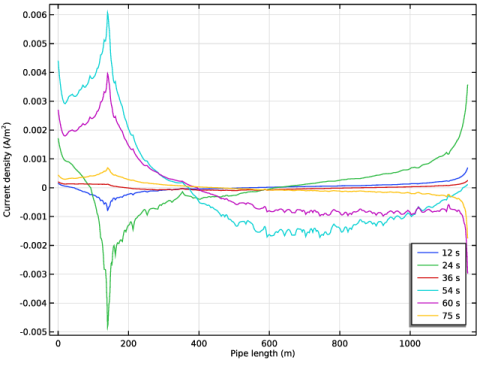
In the Settings window for 1D Plot Group, type Stray Current Density at Rail in the Label text field.
3
Locate the Plot Settings section. In the y-axis label text field, type Current density (A/m<sup>2</sup>).
4
Locate the Legend section. From the Position list, choose Lower middle.
Line Graph 1
1
In the Model Builder window, expand the Stray Current Density at Rail node, then click Line Graph 1.
2
In the Settings window for Line Graph, click Replace Expression in the upper-right corner of the y-Axis Data section. From the menu, choose Component 1 (comp1) > Cathodic Protection > Electrode kinetics > cp.iloc_er1 - Local current density - A/m².
Line Graph 2
1
In the Model Builder window, click Line Graph 2.
2
In the Settings window for Line Graph, locate the y-Axis Data section.
3
In the Expression text field, type maxop_uprail(cp.iloc_er1).
4
In the Stray Current Density at Rail toolbar, click  Plot.
Current Density at Pipe
1
In the Model Builder window, right-click Stray Current Density at Rail and choose Duplicate.
Continue with the stray current at the pipe plot (Figure 6).
2
In the Settings window for 1D Plot Group, type Current Density at Pipe in the Label text field.
3
Locate the Plot Settings section. In the x-axis label text field, type Pipe length (m).
4
Locate the Legend section. From the Position list, choose Lower right.
Line Graph 1
1
In the Model Builder window, expand the Current Density at Pipe node, then click Line Graph 1.
2
In the Settings window for Line Graph, locate the Selection section.
3
From the Selection list, choose Pipe.
4
Locate the x-Axis Data section. From the Parameter list, choose Arc length.
Line Graph 2
In the Model Builder window, right-click Line Graph 2 and choose Delete.
Line Graph 1
In the Current Density at Pipe toolbar, click  Plot.
Comparison - Corrosion Rate on Pipe at 54 s
1
In the Model Builder window, right-click Current Density at Pipe and choose Duplicate.
Continue with the plot that compares corrosion rates at the pipe (Figure 7).
2
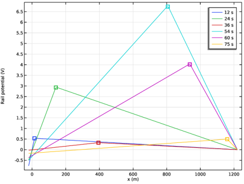
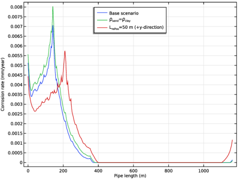
In the Settings window for 1D Plot Group, type Comparison - Corrosion Rate on Pipe at 54 s in the Label text field.
3
Locate the Data section. From the Parameter selection (L_rePos, rho_sand) list, choose All.
4
In the Parameter values (t_train (s)) list, select 54.
5
Locate the Plot Settings section. In the y-axis label text field, type Corrosion rate (mm/year).
6
Locate the Legend section. From the Position list, choose Upper middle.
Line Graph 1
1
In the Model Builder window, expand the Comparison - Corrosion Rate on Pipe at 54 s node, then click Line Graph 1.
2
In the Settings window for Line Graph, click Replace Expression in the upper-right corner of the y-Axis Data section. From the menu, choose Component 1 (comp1) > Definitions > Variables > dr_rate - Corrosion rate on pipe - m/s.
3
Locate the y-Axis Data section. From the Unit list, choose mm/yr.
4
Locate the Legends section. In the table, enter the following settings:
5
In the Comparison - Corrosion Rate on Pipe at 54 s toolbar, click  Plot.
Some of the default plots can be removed since these show little additional information.
Electrode Potential vs. Adjacent Reference (cp), Electrolyte Potential (cp)
1
In the Model Builder window, under Results, Ctrl-click to select Electrolyte Potential (cp) and Electrode Potential vs. Adjacent Reference (cp).
2
Use the Animation functionality to visualize the stray currents from the moving train better.
Animation 1
1
In the Results toolbar, click  Animation and choose Player.
2
In the Settings window for Animation, click to expand the Frames section.
3
Click the  Play button in the Graphics toolbar.