PDF

Alternating Current-Induced Corrosion
Introduction
Corrosion induced by alternating currents (AC) is evident in the oil and gas industry, particularly when a pipeline is in close proximity to high power transmission lines.
The model presented here first evaluates the effect of a direct current (DC) applied potential on corrosion using a stationary analysis, and then evaluates the effect of AC on corrosion using a transient analysis. The model is subsequently extended to investigate the effect of frequency on the AC corrosion rate, thereby demonstrating the role of the capacitive double-layer at higher frequencies.
The model is based on a paper by Ghanbari and others (Ref. 1).
Model Definition
The model geometry is defined in 1D, where the length is set to equal to the diffusion layer thickness. A steel electrode surface is assumed to be located at the left-hand side, with the bulk electrolyte boundary placed at the right, as shown in Figure 1.
Figure 1: Model geometry.
The concentration of dissolved oxygen is solved for across the diffusion layer thickness, with the transport equation defined according Fick’s law:
(1)
Here, ci is the dissolved oxygen concentration in the electrolyte (mol/m3) and Di is diffusion coefficient of dissolved oxygen in the electrolyte (m2/s).
The diffusion layer thickness is set based on the limiting current density for the oxygen reduction reaction, ilim, across the diffusion layer:
(2)
The oxygen concentration is set equal to the saturated concentration for dissolved oxygen when in equilibrium with air, csat, at the right boundary. At the electrode surface on the left, the flux of oxygen is defined based on the local current density for oxygen reduction in combination with Faraday’s law.
The Electrode Surface boundary node is used to calculate the total current density, iT,which includes contributions from the metal dissolution (anodic), oxygen reduction (cathodic) and hydrogen evolution (cathodic) electrochemical reactions, as well as the double layer capacitance.
The electrode potential is assumed to be measured versus a reference electrode located outside the diffusion layer. The electrode potential versus the reference, ET, is hence the sum of the potential drop across the electrochemical interface, E, and the potential drop across the solution resistance, Rs:
(3)
The potential drop across the electrochemical interface, E, is solved using a Global Equations node.
The potential of the steel electrode is defined to be the sum of a DC potential, EDC, and an AC potential perturbation, and is set according to
(4)
Here, ERMS is the amplitude of the AC potential; ω is the angular frequency, which is equal to 2πf, where f is the frequency of the AC potential; and t is time.
Tafel kinetics are used to define all faradaic reactions. For the oxygen reduction reaction, the kinetics expression is concentration dependent according to
(5)
where Ac is the Tafel slope and η = E − Eeq is the overpotential.
The nonfaradaic double layer capacitance current density is defined as
(6)
where Cdl is considered to be a combination of double layer and oxide capacitances. Different Cdl values are used in the model for different DC applied potentials, which are taken from Ref. 1.
The model is solved in two steps. In the first step, a stationary solution for the pure DC problem is computed. In the second time-dependent step, the solution of the stationary step is used as initial values, and the simulation is performed for multiple consecutive periods. In order to compare the AC to the DC solution, the corrosion rate is calculated as an average for the last period of the simulation.
Results and Discussion
Figure 2 shows the anodic (metal dissolution) current density for different applied DC potentials with and without AC. It can be seen that the anodic current density in both cases (with and without AC) increases with an increase in applied DC potential. Adding the AC contribution generally increases the corrosion rate, with the effect of AC being most dominant near the open circuit potential of -0.67 V/SCE.
Figure 2: Anodic current density with and without AC for different applied DC potentials.
Figure 3 and Figure 4 show the change in total current density against time along with contributions from anodic, cathodic and double layer for frequencies 60 Hz and 0.01 Hz, respectively. It can be seen that double layer (nonfaradaic) contribution to the total current density is quite significant at frequency of 60 Hz (Figure 3), whereas at lower frequency of 0.01 Hz the total current density is mainly constituted of anodic current density (faradaic).
Figure 3: Transient distribution of the total current density along with anodic, cathodic and double layer contributions at frequency of 60 Hz.
Figure 4: Transient distribution of the total current density along with anodic, cathodic and double layer contributions at frequency of 0.01 Hz.
References
1. E. Ghanbari, M. Iannuzzi, and R.S. Lillard, “The mechanism of alternating current corrosion of API grade X65 pipeline steel,” Corrosion, vol. 72, no. 9, pp. 1196–1210, 2016.
Application Library path: Corrosion_Module/General_Corrosion/ac_corrosion
Modeling Instructions
From the File menu, choose New.
New
In the New window, click  Model Wizard.
Model Wizard
1
In the Model Wizard window, click  1D.
2
In the Select Physics tree, select Electrochemistry > Electroanalysis (tcd).
3
Click Add.
4
In the Number of species text field, type 1.
5
In the Concentrations (mol/m³) table, enter the following settings:
6
In the Select Physics tree, select Mathematics > ODE and DAE Interfaces > Global ODEs and DAEs (ge).
7
Click Add.
8
Click  Study.
9
In the Select Study tree, select General Studies > Stationary.
10
Global Definitions
Load the model parameters from a text file.
Parameters 1
1
In the Model Builder window, under Global Definitions click Parameters 1.
2
In the Settings window for Parameters, locate the Parameters section.
3
Click  Load from File.
4
Geometry 1
Draw a 1D geometry representing the diffusion layer thickness.
1
From the Geometry menu, choose Interval.
Interval 1 (i1)
1
In the Model Builder window, under Component 1 (comp1) right-click Geometry 1 and choose Interval.
2
In the Settings window for Interval, locate the Interval section.
3
4
Click  Build All Objects.
Definitions
Variables 1
Load the model variables from a text file.
1
In the Definitions toolbar, click  Local Variables.
2
In the Settings window for Variables, locate the Variables section.
3
Click  Load from File.
4
Integration 1 (intop1)
Add an integration operator.
1
In the Definitions toolbar, click  Nonlocal Couplings and choose Integration.
2
In the Settings window for Integration, locate the Source Selection section.
3
From the Geometric entity level list, choose Boundary.
4
Electroanalysis (tcd)
Set up the physics of the model.
Electrolyte 1
1
In the Model Builder window, under Component 1 (comp1) > Electroanalysis (tcd) click Electrolyte 1.
2
In the Settings window for Electrolyte, locate the Diffusion section.
3
In the DcO2 text field, type D_O2.
Initial Values 1
1
In the Model Builder window, click Initial Values 1.
2
In the Settings window for Initial Values, locate the Initial Values section.
3
In the cO2 text field, type c_O2_sat.
Concentration 1
1
In the Physics toolbar, click  Boundaries and choose Concentration.
2
3
In the Settings window for Concentration, locate the Concentration section.
4
Select the Species cO2 checkbox.
5
In the c0,cO2 text field, type c_O2_sat.
Electrode Surface 1
Next, set up the Electrode Surface node to describe the anodic, cathodic, and double-layer contributions to the total current density.
1
In the Physics toolbar, click  Boundaries and choose Electrode Surface.
2
3
In the Settings window for Electrode Surface, locate the Electrode Phase Potential Condition section.
4
In the ϕs,ext text field, type E.
Electrode Reaction: Anodic Reaction
1
In the Model Builder window, click Electrode Reaction 1.
2
In the Settings window for Electrode Reaction, locate the Equilibrium Potential section.
3
From the Eeq list, choose User defined. In the associated text field, type Ecorr.
4
Locate the Electrode Kinetics section. From the Kinetics expression type list, choose Anodic Tafel equation.
5
In the i0 text field, type icorr.
6
In the Aa text field, type ba.
7
In the Label text field, type Electrode Reaction: Anodic Reaction.
Electrode Surface 1
In the Model Builder window, click Electrode Surface 1.
Electrode Reaction: Oxygen reduction cathodic reaction
1
In the Physics toolbar, click  Attributes and choose Electrode Reaction.
2
In the Settings window for Electrode Reaction, type Electrode Reaction: Oxygen reduction cathodic reaction in the Label text field.
3
Locate the Stoichiometric Coefficients section. In the n text field, type 4.
4
In the νcO2 text field, type -1.
5
Locate the Equilibrium Potential section. From the Eeq list, choose User defined. In the associated text field, type Ecorr.
6
Locate the Electrode Kinetics section. From the Kinetics expression type list, choose Cathodic Tafel equation.
7
In the i0 text field, type icorr*cO2/ c_O2_sat.
8
In the Ac text field, type bc.
Electrode Surface 1
In the Model Builder window, click Electrode Surface 1.
Electrode Reaction: Hydrogen evolution cathodic reaction
1
In the Physics toolbar, click  Attributes and choose Electrode Reaction.
2
In the Settings window for Electrode Reaction, type Electrode Reaction: Hydrogen evolution cathodic reaction in the Label text field.
3
Locate the Equilibrium Potential section. From the Eeq list, choose User defined. In the associated text field, type E_H2.
4
Locate the Electrode Kinetics section. From the Kinetics expression type list, choose Cathodic Tafel equation.
5
In the i0 text field, type i0_H2.
6
In the Ac text field, type b_H2.
Electrode Surface 1
In the Model Builder window, click Electrode Surface 1.
Double-Layer Capacitance 1
1
In the Physics toolbar, click  Attributes and choose Double-Layer Capacitance.
2
In the Settings window for Double-Layer Capacitance, locate the Double-Layer Capacitance section.
3
In the Cdl text field, type C.
Global ODEs and DAEs (ge)
Add a Global Equation to solve for electric potential, E.
Global Equations 1 (ODE1)
1
In the Model Builder window, under Component 1 (comp1) > Global ODEs and DAEs (ge) click Global Equations 1 (ODE1).
2
In the Settings window for Global Equations, locate the Global Equations section.
3
4
Locate the Units section. Click  Define Dependent Variable Unit.
5
In the Dependent variable quantity table, enter the following settings:
6
Click  Define Source Term Unit.
7
In the Source term quantity table, enter the following settings:
Study : AC Effect
1
In the Model Builder window, click Study 1.
2
In the Settings window for Study, locate the Study Settings section.
3
Clear the Generate default plots checkbox.
4
In the Label text field, type Study : AC Effect.
Parametric Sweep
Use the parametric sweep to investigate the effect of applied DC potential along with the respective double layer capacitance values.
1
In the Study toolbar, click  Parametric Sweep.
2
In the Settings window for Parametric Sweep, locate the Study Settings section.
3
4
5
6
Now solve the stationary study step to get results without AC effect first.
7
In the Study toolbar, click  Compute.
Solver Configurations
Store a copy of the solution for comparison purposes.
Solution 1 (sol1)
1
In the Model Builder window, expand the Study : AC Effect > Solver Configurations node.
2
Right-click Solution 1 (sol1) and choose Solution > Copy.
Solution 1 - No AC
1
In the Model Builder window, under Study : AC Effect > Solver Configurations click Solution 1 - Copy 1 (sol2).
2
In the Settings window for Solution, type Solution 1 - No AC in the Label text field.
Step 2: Time Dependent
Now add a Time Dependent study node to investigate the effect of AC.
1
In the Study toolbar, click  Study Steps and choose Time Dependent > Time Dependent.
2
In the Settings window for Time Dependent, locate the Study Settings section.
3
In the Output times text field, type range(0,tf/10,tf).
4
In the Study toolbar, click  Compute.
Results
Plot the anodic current density to compare the effect of AC.
Effect of AC
1
In the Results toolbar, click  1D Plot Group.
2
In the Settings window for 1D Plot Group, type Effect of AC in the Label text field.
3
Locate the Data section. From the Dataset list, choose None.
4
Click to expand the Title section. From the Title type list, choose Manual.
5
In the Title text area, type Anodic current density versus applied DC potential.
6
Locate the Plot Settings section.
7
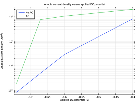
Select the y-axis label checkbox. In the associated text field, type Anodic Current density (A/m<sup>2</sup>).
8
Locate the Axis section. Select the y-axis log scale checkbox.
9
Locate the Legend section. From the Position list, choose Upper left.
Global 1
1
In the Effect of AC toolbar, click  Global.
2
In the Settings window for Global, locate the Data section.
3
From the Dataset list, choose Study : AC Effect/Solution 1 - No AC (sol2).
4
Locate the y-Axis Data section. In the table, enter the following settings:
5
Locate the x-Axis Data section. From the Parameter list, choose Expression.
6
In the Expression text field, type E_DC.
7
Click to expand the Legends section. From the Legends list, choose Manual.
8
Effect of AC
In the Model Builder window, click Effect of AC.
Global 2
1
In the Effect of AC toolbar, click  Global.
2
In the Settings window for Global, locate the Data section.
3
From the Dataset list, choose Study : AC Effect/Parametric Solutions 1 (sol4).
4
From the Time selection list, choose Last.
5
Locate the y-Axis Data section. In the table, enter the following settings:
6
Locate the x-Axis Data section. From the Axis source data list, choose Outer solutions.
7
From the Parameter list, choose Expression.
8
In the Expression text field, type E_DC.
9
Locate the Legends section. From the Legends list, choose Manual.
10
11
In the Effect of AC toolbar, click  Plot.
The plot should look like Figure 2.
Root
Next, add a new study to investigate the effect of the frequency on the corrosion using a Parametric Sweep.
Add Study
1
In the Home toolbar, click  Add Study to open the Add Study window.
2
Go to the Add Study window.
3
Find the Studies subsection. In the Select Study tree, select General Studies > Stationary.
4
Click the Add Study button in the window toolbar.
5
In the Home toolbar, click  Add Study to close the Add Study window.
Study : Frequency Effect
1
In the Settings window for Study, type Study : Frequency Effect in the Label text field.
2
Locate the Study Settings section. Clear the Generate default plots checkbox.
Step 2: Time Dependent
In the Study toolbar, click  Study Steps and choose Time Dependent > Time Dependent.
Parametric Sweep
Use the parametric sweep to investigate the effect of two frequencies, 60[Hz] and 0.01[Hz].
1
In the Study toolbar, click  Parametric Sweep.
2
In the Settings window for Parametric Sweep, locate the Study Settings section.
3
4
Step 2: Time Dependent
1
In the Model Builder window, click Step 2: Time Dependent.
2
In the Settings window for Time Dependent, locate the Study Settings section.
3
In the Output times text field, type range(0,tf/10,tf).
4
In the Study toolbar, click  Compute.
Results
Now, plot the total current density along with different contributions for different frequencies.
Effect of AC Frequency
1
In the Results toolbar, click  1D Plot Group.
2
In the Settings window for 1D Plot Group, type Effect of AC Frequency in the Label text field.
3
Locate the Data section. From the Dataset list, choose Study : Frequency Effect/Parametric Solutions 2 (sol11).
4
From the Parameter selection (f) list, choose From list.
5
In the Parameter values (f (Hz)) list, select 60.
6
Locate the Title section. From the Title type list, choose Manual.
7
In the Title text area, type Current Density Versus Time.
8
Locate the Plot Settings section.
9
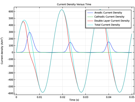
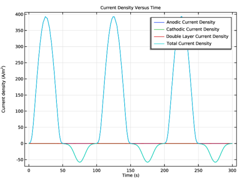
Select the y-axis label checkbox. In the associated text field, type Current density (A/m<sup>2</sup>).
Point Graph: Anodic Current Density
1
In the Effect of AC Frequency toolbar, click  Point Graph.
2
In the Settings window for Point Graph, type Point Graph: Anodic Current Density in the Label text field.
3
4
Click Replace Expression in the upper-right corner of the y-Axis Data section. From the menu, choose Component 1 (comp1) > Electroanalysis > Electrode kinetics > tcd.iloc_er1 - Local current density - A/m².
5
Click to expand the Legends section. Select the Show legends checkbox.
6
From the Legends list, choose Manual.
7
Point Graph: Cathodic Current Density
1
Right-click Point Graph: Anodic Current Density and choose Duplicate.
2
In the Settings window for Point Graph, type Point Graph: Cathodic Current Density in the Label text field.
3
Locate the y-Axis Data section. In the Expression text field, type tcd.iloc_er2+tcd.iloc_er3.
4
Locate the Legends section. In the table, enter the following settings:
Point Graph: Double Layer Current Density
1
Right-click Point Graph: Cathodic Current Density and choose Duplicate.
2
In the Settings window for Point Graph, locate the y-Axis Data section.
3
In the Expression text field, type tcd.idl.
4
In the Label text field, type Point Graph: Double Layer Current Density.
5
Locate the Legends section. In the table, enter the following settings:
Point Graph: Total Current Density
1
Right-click Point Graph: Double Layer Current Density and choose Duplicate.
2
In the Settings window for Point Graph, click Replace Expression in the upper-right corner of the y-Axis Data section. From the menu, choose Component 1 (comp1) > Electroanalysis > Electrode kinetics > tcd.itot - Total interface current density - A/m².
3
In the Label text field, type Point Graph: Total Current Density.
4
Locate the Legends section. In the table, enter the following settings:
Effect of AC Frequency
1
In the Model Builder window, click Effect of AC Frequency.
2
In the Effect of AC Frequency toolbar, click  Plot.
The plot should look like Figure 3.
Now plot current density contributions at 0.01 Hz.
3
In the Settings window for 1D Plot Group, locate the Data section.
4
In the Parameter values (f (Hz)) list, select 0.01.
5
In the Effect of AC Frequency toolbar, click  Plot.
The plot should look like Figure 4.