|
|
|
|
•
|
|
•
|
|
•
|
|
•
|


|
1
|
|
2
|
|
4
|
|
1
|
Go to the Select System window.
|
|
2
|
|
3
|
Click the Next button in the window toolbar.
|
|
1
|
Go to the Select Species window.
|
|
2
|
|
3
|
Click
|
|
4
|
|
5
|
Click
|
|
6
|
Click the Next button in the window toolbar.
|
|
1
|
Go to the Select Thermodynamic Model window.
|
|
2
|
From the list, choose UNIFAC VLE.
|
|
3
|
Click the Finish button in the window toolbar.
|
|
1
|
Go to the Select Species window.
|
|
2
|
In the list, select chloroform.
|
|
3
|
Click
|
|
4
|
In the list, select methanol.
|
|
5
|
Click
|
|
6
|
Click the Next button in the window toolbar.
|
|
1
|
Go to the Equilibrium Specifications window.
|
|
2
|
|
3
|
|
4
|
|
5
|
Click the Next button in the window toolbar.
|
|
1
|
Go to the Equilibrium Function Overview window.
|
|
2
|
Click the Finish button in the window toolbar.
|
|
1
|
|
2
|
|
1
|
|
2
|
Go to the Add Study window.
|
|
3
|
Find the Studies subsection. In the Select Study tree, select Preset Studies for Selected Physics Interfaces > Stationary.
|
|
4
|
Click the Add Study button in the window toolbar.
|
|
5
|
|
1
|
In the Model Builder window, under Study 1 - Dew Point and Boiling Point Curves click Step 1: Stationary.
|
|
2
|
|
3
|
Select the Auxiliary sweep checkbox.
|
|
4
|
|
5
|
Click
|
|
7
|
|
1
|
|
2
|
|
3
|
|
4
|
Locate the Plot Settings section.
|
|
5
|
|
6
|
|
1
|
|
2
|
|
4
|
|
5
|
|
6
|
Click to expand the Coloring and Style section. Find the Line style subsection. From the Line list, choose Cycle.
|
|
7
|
|
8
|
|
1
|
|
2
|
|
3
|
|
4
|
|
5
|
|
6
|
|
7
|
|
1
|
|
2
|
|
3
|
Select the Manual axis limits checkbox.
|
|
4
|
|
5
|
|
6
|
|
1
|
|
2
|
|
1
|
|
2
|
|
1
|
|
2
|
Go to the Add Physics window.
|
|
3
|
|
4
|
Find the Physics interfaces in study subsection. In the table, clear the Solve checkbox for Study 1 - Dew Point and Boiling Point Curves.
|
|
5
|
Click the Add to Component 1 button in the window toolbar.
|
|
6
|
|
1
|
In the Model Builder window, expand the Component 1 (comp1) > Global ODEs and DAEs (ge) > Global Equations 1 (ODE1) node, then click Global Equations 1 (ODE1).
|
|
2
|
|
4
|
|
5
|
Click
|
|
6
|
|
7
|
|
8
|
Click OK.
|
|
9
|
|
1
|
Go to the Select Properties window.
|
|
2
|
|
3
|
In the list, select Enthalpy (J/mol).
|
|
4
|
Click
|
|
5
|
Click the Next button in the window toolbar.
|
|
1
|
Go to the Select Phase window.
|
|
2
|
Click the Next button in the window toolbar.
|
|
1
|
Go to the Select Species window.
|
|
2
|
Click
|
|
3
|
Click the Next button in the window toolbar.
|
|
1
|
Go to the Mixture Property Overview window.
|
|
2
|
Click the Finish button in the window toolbar.
|
|
1
|
Go to the Select Properties window.
|
|
2
|
In the list, select Enthalpy (J/mol).
|
|
3
|
Click
|
|
4
|
Click the Next button in the window toolbar.
|
|
1
|
Go to the Select Phase window.
|
|
2
|
From the list, choose Liquid.
|
|
3
|
Click the Next button in the window toolbar.
|
|
1
|
Go to the Select Species window.
|
|
2
|
Click
|
|
3
|
Click the Next button in the window toolbar.
|
|
1
|
Go to the Mixture Property Overview window.
|
|
2
|
Click the Finish button in the window toolbar.
|
|
1
|
|
2
|
|
1
|
In the Model Builder window, under Component 1 (comp1) right-click Definitions and choose Variables.
|
|
2
|
|
1
|
|
2
|
Go to the Add Study window.
|
|
3
|
|
4
|
Right-click and choose Add Study.
|
|
5
|
|
1
|
|
2
|
Select the Auxiliary sweep checkbox.
|
|
3
|
Click
|
|
6
|
Click
|
|
8
|
|
9
|
|
10
|
|
11
|
|
12
|
|
13
|
|
1
|
|
2
|
|
3
|
Select the Only plot when requested checkbox.
|
|
1
|
|
2
|
|
3
|
|
1
|
|
2
|
|
3
|
|
4
|
|
5
|
Locate the y-Axis Data section. In the table, enter the following settings:
|
|
6
|
|
7
|
Locate the Coloring and Style section. Find the Line style subsection. From the Line list, choose Dashed.
|
|
8
|
|
9
|
|
10
|
Clear the Solution checkbox.
|
|
11
|
Clear the Description checkbox.
|
|
1
|
|
2
|
|
3
|
|
4
|
|
5
|
Locate the y-Axis Data section. In the table, enter the following settings:
|
|
6
|
|
7
|
Locate the Coloring and Style section. Find the Line style subsection. From the Line list, choose Dotted.
|
|
8
|
|
9
|
|
10
|
Clear the Solution checkbox.
|
|
11
|
Clear the Description checkbox.
|
|
1
|
|
2
|
|
3
|
|
4
|
Select the y-axis label checkbox. In the associated text field, type Enthalpy / kJ \cdot mol<sup>-1</sup>.
|
|
1
|
|
2
|
|
3
|
|
4
|
Locate the y-Axis Data section. In the table, enter the following settings:
|
|
5
|
|
6
|
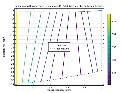
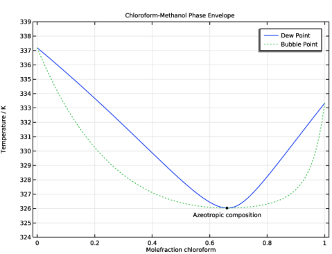
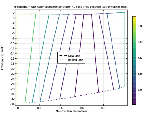
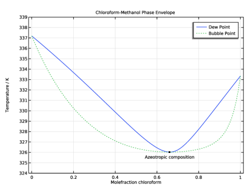
In the Title text area, type H-x diagram with color coded temperature (K). Solid lines describe isothermal tie lines..
|
|
7
|
|
8
|
|
9
|
|
10
|
|
1
|
|
2
|
|
3
|
|
4
|
|
5
|
Clear the Color legend checkbox.
|
|
6
|
|
1
|
|
2
|
|
3
|
|
1
|
|
2
|
|
3
|
|
4
|
Click to expand the Title section. Locate the Coloring and Style section. Select the Color legend checkbox.
|
|
5
|