PDF

A 3D Model of a Diesel Particulate Filter
Introduction
This example studies the averaged flow field, concentration, and temperature distribution in a homogenized model of a diesel particulate filter (DPF). The filter consists of a series of parallel channels that are closed off in an alternating fashion. The walls shared by neighboring channels are porous, allowing gas to pass through them while at the same time separating particles from the flow (Figure 1).
Figure 1: Drawing of a diesel particulate filter. At the reactor’s inlet the outlet channel is closed, while at the reactor’s outlet the inlet channel is closed.
Several factors influence a DPF’s efficiency and durability. Important issues include the removal of soot particles from the filter membranes and the influence of thermal stress on the ceramic structure, stress that arises during repeated operating cycles. Mathematical modeling provides a powerful tool for investigating such critical parameters under a wide range of operating conditions.
This example sets up and solves the coupled flow plus mass and thermal transport equations describing the transport/reaction phenomena in a diesel particulate filter. An important aspect it illustrates is how you can tailor the predefined application modes of COMSOL Multiphysics to represent a specialized mathematical model.
Model Definition
In a detailed DPF model, you can treat the channels and porous membrane with their true geometry with the only simplification being the membrane description. The membrane could, for example, be described with a porous-media approach using effective transport properties. Flow in the channels is expected to be close to fully developed laminar flow although there could be a slight deviation due to the relatively small flow of fluid over the membrane from the inlet to the outlet channels.
Figure 2: Cross section of a unit cell consisting of an inlet and an outlet channel separated by a porous membrane.
In general, a detailed model of the flow in the hundreds or even thousands of channels that make up a full filter geometry is not feasible due to the demands on computer capability. However, a homogenized model is realizable. Using such an approach, assume that the velocity profile is that of a fully developed laminar flow. The average flow rate in a cross section of one channel is proportional to the pressure gradient in the channel:
(1)
Here u denotes the flow velocity (m/s), kl represents a lumped friction factor (m2/(Pa·s)), and p is the pressure (Pa).
Velocity and Pressure
You can obtain the average velocity in the inlet channel from a mass balance. The velocity in this channel decreases as gas passes through the porous membrane to the outlet channel. The crossover of gas from an inlet to an outlet channel is assumed to be proportional to the pressure difference across the membrane.
Figure 3 shows the geometric unit cell used to set up the balance equations.
Figure 3: Geometric unit cell for the homogenized DPF model. Each inlet channel has porous walls in common with four outlet channels and vice versa.
For an inlet channel, the balance equation with respect to mass flow becomes
(2)
where κm denotes the porous membrane’s permeability (m2), H is the channel height (m), η denotes the fluid’s viscosity (Pa·s), δm gives the membrane’s thickness (m), p1 represents the pressure in the inlet channel (Pa), and p2 equals the pressure in the outlet channel (Pa).
The density is a function of pressure according to the ideal gas law:
(3)
Here M1 denotes the fluid’s average molecular weight (kg/mol), Rg is the gas constant (J/(mol·K)), and T1 gives the temperature in the inlet channel (K).
The corresponding equation for the outlet channel is
(4)
Note that the source/sink terms in Equation 2 and Equation 4 are proportional to the volumetric flow through the membrane per unit area, or the superficial velocity:
(5)
The pressure fields and thus also this velocity field vary only in the x direction, and each inlet channel is separated from the other inlet channels by an impermeable wall. The inlet and outlet pressures connect the array of inlet channels to each other. If the porous membrane’s permeability, encoded in the variable κm, varies in the filter, a corresponding distribution of the superficial velocity in the inlet and outlet channels results. In addition, the temperature field is connected for the entire system, and heat flows between the different unit cells. For this reason it is appropriate to expand the 1D model to a 3D model that accounts for the impermeability of the walls separating the inlet and outlet channels in adjacent unit cells.
You can express this impermeability with a diagonal friction tensor, k, where only the xx component is nonzero and equal to kl. The model equations then read
(6)
and
(7)
These equations are valid if the permeability and thickness of the porous membrane are constant throughout the process, which is not the case when soot particles deposit on the membrane surface. However, you can derive a model analogous to the one just described by assuming that two porous membranes separate the outlet and inlet channels, one formed by the soot layer and the second one being the porous membrane just described. This approach results in the following equations:
(8)
and
(9)
Here a and b are defined by the equations
(10)
(11)
where κs denotes the soot layer’s permeability (m2), and δs equals its thickness (m). The superficial flow velocity through the membrane is now given by
(12)
At the filter entrance, the boundary condition for the inlet channels specifies a given pressure. All other boundaries are insulating, that is,
(13)
where n denotes the normal vector to the boundary.
The boundary conditions for the outlet channels specify the pressure at the filter exit and impose insulation at all other boundaries:
(14)
Mass Balances
The soot particles are present only in the inlet channel because they are deposited as a film on the porous membrane. A balance for soot particles introduces the deposition of soot particles as a sink to the flux of particles in the open channel. This gives the transport equation
(15)
where  cs denotes the soot-particle concentration (mol/m3), and Ds is the diffusivity of soot particles (m2/s).
The model defines the concentration of oxygen using two mass balances, one for the inlet and another for the outlet channel. The mass balance in the inlet channel contains the term where oxygen reacts in the combustion reaction with soot. The mass balance in the inlet channel is represented by the equation
(16)
where co2 denotes the oxygen concentration (mol/m3), Do2 gives the diffusion coefficient (m2/s), and Rs equals the reaction rate for the surface reaction (mol/(m2·s)).
The corresponding balance for oxygen in the outlet channel yields
(17)
Note the addition of the flow term of oxygen over the membrane as a source term in the outlet channel balance.
The balance of soot results in an expression for the growth or consumption of the soot layer:
(18)
where δs denotes the soot layer’s thickness (m), ρs represents its effective density (kg/m3), and Ms equals the molecular weight of carbon (kg/mol).
The boundary condition for co2,1 sets the concentration at the inlet, while insulation is used for all other boundaries. For co2,2, use a convective flux condition at the outlet and set all other boundaries to insulation. The initial conditions for both co2,1 and co2,2 are 0.
Energy Balance
The energy balance in the reactor consists of three equations: one for the inlet channels, one for the porous membranes, and one for the outlet channels.
The balance for the inlet channels reads
(19)
(20)
where T1 is the temperature in the inlet channels (K), Tm is the temperature in the membrane (K), Cp1 gives the heat capacity of the gas in the inlet channel (J/(kg·K)), h equals the heat transfer coefficient (W/(m2·K)), and q1 is the flux vector.
In the membrane, the energy equation is given by
(21) 
(22)
Here the subscript “m” refers to the membrane so that Tm is its temperature, T2 equals the temperature in the outlet channels (K), Cp2 refers to the heat capacity of the gas in the outlet channels (J/(kg·K)), and h is the heat transfer coefficient between the membrane and the channels.
The last equation determines the temperature in the outlet channel:
(23)
(24)
The boundary conditions for the inlet channel are a given temperature at the inlet and insulation at all other boundaries. At the outlet channel, use a convective flux condition at the outlet and set all other boundaries to insulation. The initial condition specifies a temperature equal to the inlet temperature of the gas.
For the membrane, the heat flux through the boundaries is given by
(25)
where houter denotes the heat transfer coefficient, and Tamb equals the ambient temperature. The initial temperature is set equal to the inlet temperature.
Homogenized Filter Geometry
The balance equations covered above are implemented on a 3D filter geometry. The cross section of the filter is an oval, 5.86 inches in width, 4.66 inches in height, and the length of the filter is 8 inches. Mirror symmetry reduces the geometry to one quarter of the filter.
Figure 4: Symmetry reduces the modeling geometry to one quarter of the full filter.
Mesh
Boundary layer meshing is used to create a denser mesh in the radial direction of the filter, near the outer surface. When extruding the cross sectional mesh you can further control the distribution to get a denser mesh near the filter inlet and outlet.
Figure 5: Boundary layer meshing and mesh extrusion make it possible to efficiently discretize the geometry.
Results and Discussion
Figure 6 shows the gas velocity along the inlet and outlet filter channels. At the start of the simulation (t = 0), a 25-μm layer of soot is evenly distributed on top of the porous membranes of the inlet channels. The pressure difference over the filter is 50 Pa.
The top panel in Figure 7 shows the pressure difference (p1 – p2) across an inlet/outlet channel pair located at the center of the filter. The bottom panel illustrates the buildup of soot during 15 minutes of simulated operation with no carbon oxidation present. As expected, soot builds up primarily at the channel’s entrance and end, because this is where the pressure gradient and, consequently, the trans-membrane velocity have their highest values.
Figure 6: Gas velocity (m/s) in the inlet channels (v1, top) and outlet channels (v2, bottom).
Figure 7: Pressure difference (top) and soot-layer thickness (bottom) along a channel located at the filter centerline. No soot oxidation is present.
The top image of Figure 8 shows the filter temperature distribution, Tm, when the inlet gas temperature is 550 K, and the ambient temperature is set to 300 K. Furthermore, the effect of soot oxidation is disregarded. The temperature gradients due to cooling of the filter’s outer surface are evident. The bottom image shows Tm, when soot oxidation is taken into account. Filter temperatures exceeding that of the inlet gas are observed in the front end of the filter.
Figure 9 illustrates the time evolution of the soot layer’s thickness (0–900 s). The layer grows due to the deposition of particles from the gas phase, and it is removed by oxidation. Results are shown for a channel located at the filter periphery (top) and at the center of the filter (bottom).
Figure 8: Filter temperature, Tm, when no oxidation takes place (top), and when soot oxidation is taken into account (bottom).
Figure 9: Soot-layer thickness along a channel located at the filter periphery (top) and at the filter centerline (bottom).
Clearly, soot removal is less efficient in the peripheral parts of the filter as lower temperature in these areas decreases the oxidation rate significantly.
Finally, Figure 10 shows the pressure drop across a centrally placed channel pair as function of time (0–900 s). In accordance with the diminishing soot layer illustrated in Figure 9, the pressure drop is reduced in the front end of the filter.
Figure 10: The pressure drop across a centrally placed channel pair is affected by the diminishing soot layer.
Application Library path: Chemical_Reaction_Engineering_Module/Reactors_with_Porous_Catalysts/diesel_particulate_filter
Modeling Instructions
From the File menu, choose New.
New
In the New window, click  Model Wizard.
Model Wizard
1
In the Model Wizard window, click  3D.
Add one Chemistry, three Transport of Diluted Species, two Darcy’s Law, three Heat Transfer in Fluids, and one General Form PDE interfaces.
2
In the Select Physics tree, select Chemical Species Transport > Chemistry (chem).
3
Click Add.
4
In the Select Physics tree, select Chemical Species Transport > Transport of Diluted Species (tds).
5
Click Add.
6
In the Concentrations (mol/m³) table, enter the following settings:
7
Click Add.
8
In the Concentrations (mol/m³) table, enter the following settings:
9
Click Add.
10
In the Concentrations (mol/m³) table, enter the following settings:
11
In the Select Physics tree, select Fluid Flow > Porous Media and Subsurface Flow > Darcy’s Law (dl).
12
Click Add.
13
In the Pressure (Pa) text field, type p1.
14
Click Add.
15
In the Pressure (Pa) text field, type p2.
16
In the Select Physics tree, select Heat Transfer > Heat Transfer in Fluids (ht).
17
Click Add.
18
In the Temperature (K) text field, type T1.
19
Click Add.
20
In the Temperature (K) text field, type Tm.
21
Click Add.
22
In the Temperature (K) text field, type T2.
23
In the Select Physics tree, select Mathematics > PDE Interfaces > General Form PDE (g).
24
Click Add.
25
In the Field name (1) text field, type ds.
26
In the Dependent variables (1) table, enter the following settings:
27
Click  Select Dependent Variable Quantity.
28
In the Physical Quantity dialog, type length in the text field.
29
In the tree, select General > Length (m).
30
31
In the Model Wizard window, click  Select Source Term Quantity.
32
In the Physical Quantity dialog, type velocity in the text field.
33
In the tree, select General > Velocity (m/s).
34
35
In the Model Wizard window, click  Study.
36
In the Select Study tree, select General Studies > Stationary.
37
Global Definitions
Load the model parameters from a text file.
Parameters 1
1
In the Model Builder window, under Global Definitions click Parameters 1.
2
In the Settings window for Parameters, locate the Parameters section.
3
Click  Load from File.
4
Definitions
Load the variable definitions from a text file.
Variables 1
1
In the Model Builder window, under Component 1 (comp1) right-click Definitions and choose Variables.
2
In the Settings window for Variables, locate the Variables section.
3
Click  Load from File.
4
Geometry 1
Work Plane 1 (wp1)
1
In the Geometry toolbar, click  Work Plane.
2
In the Settings window for Work Plane, locate the Plane Definition section.
3
From the Plane list, choose yz-plane.
Work Plane 1 (wp1) > Plane Geometry
1
In the Model Builder window, click Plane Geometry.
2
In the Settings window for Plane Geometry, locate the Visualization section.
3
Find the In-plane visualization of 3D geometry subsection. Clear the Coincident entities (blue) checkbox.
4
Clear the Intersection (green) checkbox.
Work Plane 1 (wp1) > Ellipse 1 (e1)
1
In the Work Plane toolbar, click  Ellipse.
2
In the Settings window for Ellipse, locate the Size and Shape section.
3
In the a-semiaxis text field, type 5.86[in].
4
In the b-semiaxis text field, type 4.66[in].
5
In the Sector angle text field, type 90.
Symmetry allows you to reduce the cross section to one quarter of the ellipse.
Extrude 1 (ext1)
1
In the Model Builder window, right-click Geometry 1 and choose Extrude.
2
In the Settings window for Extrude, locate the Distances section.
3
4
Click  Build All Objects.
5
Click the  Zoom Extents button in the Graphics toolbar.
Chemistry (chem)
Because the reaction happens in the soot layer, couple the reaction temperature to the temperature from the Heat Transfer in Fluids interface on the soot layer.
1
In the Model Builder window, under Component 1 (comp1) click Chemistry (chem).
2
In the Settings window for Chemistry, locate the Model Input section.
3
From the T list, choose Temperature (ht2).
Reaction 1
The reaction happens on the surface of the catalyst.
1
In the Physics toolbar, click  Domains and choose Reaction.
2
In the Settings window for Reaction, locate the Reaction Formula section.
3
In the Formula text field, type C+O2+CexOy(ads)=>CO2+CexOy(ads).
4
Click Apply.
5
Locate the Reaction Rate section. From the list, choose User defined.
6
In the rj text field, type Rs_factor*chem.kf_1*chem.c_O2.
7
Locate the Reaction Orders section. Find the Volumetric overall reaction order subsection. In the Forward text field, type 1.
8
Find the Surface overall reaction order subsection. In the Forward text field, type 0.
The Rs_factor in the above Reaction rate expression will be used in the Parametric Sweep to study the model with and without oxidation reaction.
9
Locate the Rate Constants section. Select the Use Arrhenius expressions checkbox.
10
In the Af text field, type Af.
11
In the Ef text field, type Ef.
Assume that the enthalpy of reaction is constant, independent of temperature.
12
Locate the Reaction Thermodynamic Properties section. From the Enthalpy of reaction list, choose User defined.
13
In the H text field, type H_ox.
Surface species: CexOy(ads)
The site density on the catalyst surface is held constant.
1
In the Model Builder window, click Surface species: CexOy(ads).
2
In the Settings window for Species, click to expand the Constant Concentration/Activity section.
3
Select the Keep concentration/activity constant checkbox.
The oxygen concentration in the reaction is set equal to that in the inlet channel (c1_O2).
4
In the Model Builder window, click Chemistry (chem).
5
In the Settings window for Chemistry, locate the Species Matching section.
6
Find the Bulk species subsection. From the Species solved for list, choose Transport of Diluted Species.
7
8
Find the Surface species subsection. In the table, enter the following settings:
9
Click the  Show More Options button in the Model Builder toolbar.
10
In the Show More Options dialog, in the tree, select the checkbox for the node Physics > Advanced Physics Options.
11
Transport of Diluted Species (tds)
1
In the Model Builder window, under Component 1 (comp1) click Transport of Diluted Species (tds).
2
In the Settings window for Transport of Diluted Species, click to expand the Advanced Settings section.
3
From the Material balance form list, choose Conservative.
Fluid 1
1
In the Model Builder window, under Component 1 (comp1) > Transport of Diluted Species (tds) click Fluid 1.
2
In the Settings window for Fluid, locate the Convection section.
3
Specify the u vector as
4
Locate the Diffusion section. From the list, choose Diagonal.
5
Specify the Dc1O2 matrix as
Reactions 1
1
In the Physics toolbar, click  Domains and choose Reactions.
The mass source of oxygen consists of two parts: one from the reaction and the other from the outflow to the soot layer (or membrane).
2
3
In the Settings window for Reactions, locate the Reaction Rates section.
4
In the Rc1O2 text field, type -(4/H)*v_m*c1_O2+(4/H)*chem.Rsurf_O2.
Inflow 1
1
In the Physics toolbar, click  Boundaries and choose Inflow.
2
3
In the Settings window for Inflow, locate the Concentration section.
4
In the c0,c1O2 text field, type c_O2_in.
Transport of Diluted Species 2 (tds2)
1
In the Model Builder window, under Component 1 (comp1) click Transport of Diluted Species 2 (tds2).
2
In the Settings window for Transport of Diluted Species, click to expand the Advanced Settings section.
3
From the Material balance form list, choose Conservative.
Fluid 1
1
In the Model Builder window, under Component 1 (comp1) > Transport of Diluted Species 2 (tds2) click Fluid 1.
2
In the Settings window for Fluid, locate the Convection section.
3
Specify the u vector as
4
Locate the Diffusion section. From the list, choose Diagonal.
5
Specify the Dc2C matrix as
Initial Values 1
1
In the Model Builder window, click Initial Values 1.
2
In the Settings window for Initial Values, locate the Initial Values section.
3
In the c2C text field, type c_s0.
Reactions 1
1
In the Physics toolbar, click  Domains and choose Reactions.
2
3
In the Settings window for Reactions, locate the Reaction Rates section.
4
In the Rc2C text field, type -(4/H)*c2_C*v_m.
Concentration 1
1
In the Physics toolbar, click  Boundaries and choose Concentration.
2
3
In the Settings window for Concentration, locate the Concentration section.
4
Select the Species c2_C checkbox.
5
In the c0,c2C text field, type c_s0.
Transport of Diluted Species 3 (tds3)
1
In the Model Builder window, under Component 1 (comp1) click Transport of Diluted Species 3 (tds3).
2
In the Settings window for Transport of Diluted Species, click to expand the Advanced Settings section.
3
From the Material balance form list, choose Conservative.
Fluid 1
1
In the Model Builder window, under Component 1 (comp1) > Transport of Diluted Species 3 (tds3) click Fluid 1.
2
In the Settings window for Fluid, locate the Convection section.
3
Specify the u vector as
4
Locate the Diffusion section. From the list, choose Diagonal.
5
Specify the Dc3O2 matrix as
Reactions 1
1
In the Physics toolbar, click  Domains and choose Reactions.
2
3
In the Settings window for Reactions, locate the Reaction Rates section.
4
In the Rc3O2 text field, type (4/H)*v_m*c1_O2.
Compared to the inlet channel, there is no reaction source term in the outlet channel.
Outflow 1
1
In the Physics toolbar, click  Boundaries and choose Outflow.
2
Darcy’s Law (dl)
Fluid 1
1
In the Model Builder window, under Component 1 (comp1) > Darcy’s Law (dl) > Porous Medium 1 click Fluid 1.
2
In the Settings window for Fluid, locate the Fluid Properties section.
3
From the ρ list, choose User defined. In the associated text field, type rho1.
4
From the μ list, choose User defined. In the associated text field, type eta.
Porous Matrix 1
1
In the Model Builder window, click Porous Matrix 1.
2
In the Settings window for Porous Matrix, locate the Matrix Properties section.
3
From the εp list, choose User defined. In the associated text field, type 1.
4
From the κ list, choose User defined. In the associated text field, type k_l*eta.
Mass Source 1
1
In the Physics toolbar, click  Domains and choose Mass Source.
2
In the Settings window for Mass Source, locate the Domain Selection section.
3
From the Selection list, choose All domains.
4
Locate the Mass Source section. In the Qm text field, type -rho1*(p1-p2)*a*b/(a+b).
Pressure 1
1
In the Physics toolbar, click  Boundaries and choose Pressure.
2
3
In the Settings window for Pressure, locate the Pressure section.
4
In the p0 text field, type p_inlet.
Darcy’s Law 2 (dl2)
Fluid 1
1
In the Model Builder window, under Component 1 (comp1) > Darcy’s Law 2 (dl2) > Porous Medium 1 click Fluid 1.
2
In the Settings window for Fluid, locate the Fluid Properties section.
3
From the ρ list, choose User defined. In the associated text field, type rho2.
4
From the μ list, choose User defined. In the associated text field, type eta.
Porous Matrix 1
1
In the Model Builder window, click Porous Matrix 1.
2
In the Settings window for Porous Matrix, locate the Matrix Properties section.
3
From the εp list, choose User defined. In the associated text field, type 1.
4
From the κ list, choose User defined. In the associated text field, type k_l*eta.
Mass Source 1
1
In the Physics toolbar, click  Domains and choose Mass Source.
2
3
In the Settings window for Mass Source, locate the Mass Source section.
4
In the Qm text field, type rho2*(p1-p2)*a*b/(a+b).
Pressure 1
1
In the Physics toolbar, click  Boundaries and choose Pressure.
2
3
In the Settings window for Pressure, locate the Pressure section.
4
In the p0 text field, type p_outlet.
Heat Transfer in Fluids (ht)
Fluid 1
1
In the Model Builder window, under Component 1 (comp1) > Heat Transfer in Fluids (ht) click Fluid 1.
2
In the Settings window for Fluid, locate the Heat Convection section.
3
Specify the u vector as
4
Locate the Heat Conduction, Fluid section. From the k list, choose User defined. From the list, choose Diagonal.
5
Specify the k matrix as
6
Locate the Thermodynamics, Fluid section. From the Fluid type list, choose Gas/Liquid.
7
From the ρ list, choose User defined. In the associated text field, type rho1.
8
From the Cp list, choose User defined. In the associated text field, type Cp_gas.
9
From the γ list, choose User defined.
Initial Values 1
1
In the Model Builder window, click Initial Values 1.
2
In the Settings window for Initial Values, locate the Initial Values section.
3
In the T1 text field, type T0.
Heat Source 1
1
In the Physics toolbar, click  Domains and choose Heat Source.
The heat source is contributed by the fluid flow and the heat transfer caused by the temperature difference between the inlet channel and the soot layer (or membrane).
2
3
In the Settings window for Heat Source, locate the Heat Source section.
4
In the Q0 text field, type -(4/H)*rho1*Cp_gas*T1*v_m-(4/H)*ht_fg*(T1-Tm).
Temperature 1
1
In the Physics toolbar, click  Boundaries and choose Temperature.
2
3
In the Settings window for Temperature, locate the Temperature section.
4
In the T0 text field, type T_inlet.
Heat Transfer in Fluids 2 (ht2)
Fluid 1
1
In the Model Builder window, under Component 1 (comp1) > Heat Transfer in Fluids 2 (ht2) click Fluid 1.
2
In the Settings window for Fluid, locate the Heat Conduction, Fluid section.
3
From the k list, choose User defined. From the list, choose Diagonal.
4
Specify the k matrix as
5
Locate the Thermodynamics, Fluid section. From the Fluid type list, choose Gas/Liquid.
6
From the ρ list, choose User defined. In the associated text field, type rho_m.
7
From the Cp list, choose User defined. In the associated text field, type Cp_m.
8
From the γ list, choose User defined.
Initial Values 1
1
In the Model Builder window, click Initial Values 1.
2
In the Settings window for Initial Values, locate the Initial Values section.
3
In the Tm text field, type T0.
Heat Source 1
1
In the Physics toolbar, click  Domains and choose Heat Source.
2
3
In the Settings window for Heat Source, locate the Heat Source section.
4
In the Q0 text field, type (chem.Qs+(rho1*T1-rho2*T2)*Cp_gas*v_m-ht_fg*(2*Tm-T1-T2))/d_m.
The heat source is determined by fluid inflow from the inlet channel, fluid outflow to the outlet channel, and heat transfer caused by the temperature differences between the soot layer, inlet channel, and outlet channel.
Heat Flux 1
1
In the Physics toolbar, click  Boundaries and choose Heat Flux.
2
3
In the Settings window for Heat Flux, locate the Heat Flux section.
4
In the q0 text field, type -ht_fg*(Tm-T1).
Heat Flux 2
1
In the Physics toolbar, click  Boundaries and choose Heat Flux.
2
3
In the Settings window for Heat Flux, locate the Heat Flux section.
4
In the q0 text field, type -ht_fa*(Tm-T_amb).
Heat Flux 3
1
In the Physics toolbar, click  Boundaries and choose Heat Flux.
2
3
In the Settings window for Heat Flux, locate the Heat Flux section.
4
In the q0 text field, type -ht_fg*(Tm-T2).
Heat Transfer in Fluids 3 (ht3)
Fluid 1
1
In the Model Builder window, under Component 1 (comp1) > Heat Transfer in Fluids 3 (ht3) click Fluid 1.
2
In the Settings window for Fluid, locate the Heat Convection section.
3
Specify the u vector as
4
Locate the Heat Conduction, Fluid section. From the k list, choose User defined. From the list, choose Diagonal.
5
Specify the k matrix as
6
Locate the Thermodynamics, Fluid section. From the Fluid type list, choose Gas/Liquid.
7
From the ρ list, choose User defined. In the associated text field, type rho2.
8
From the Cp list, choose User defined. In the associated text field, type Cp_gas.
9
From the γ list, choose User defined.
Initial Values 1
1
In the Model Builder window, click Initial Values 1.
2
In the Settings window for Initial Values, locate the Initial Values section.
3
In the T2 text field, type T0.
Heat Source 1
1
In the Physics toolbar, click  Domains and choose Heat Source.
2
3
In the Settings window for Heat Source, locate the Heat Source section.
4
In the Q0 text field, type (4/H)*rho2*Cp_gas*Tm*v_m-(4/H)*ht_fg*(T2-Tm).
Outflow 1
1
In the Physics toolbar, click  Boundaries and choose Outflow.
2
General Form PDE (g)
General Form PDE 1
1
In the Model Builder window, under Component 1 (comp1) > General Form PDE (g) click General Form PDE 1.
2
In the Settings window for General Form PDE, locate the Conservative Flux section.
3
Specify the Γ vector as
Here, dsx, dsy, and dsz are the ds gradients along the x, y, and z directions, respectively.
4
Locate the Source Term section. In the f text field, type (chem.Rsurf_C+c2_C*v_m)*M_s/rho_s.
Initial Values 1
1
In the Model Builder window, click Initial Values 1.
2
In the Settings window for Initial Values, locate the Initial Values section.
3
In the ds text field, type ds0.
Mesh 1
Free Triangular 1
1
In the Mesh toolbar, click  More Generators and choose Free Triangular.
2
Size 1
1
Right-click Free Triangular 1 and choose Size.
2
In the Settings window for Size, locate the Element Size section.
3
From the Predefined list, choose Finer.
Boundary Layers 1
1
In the Mesh toolbar, click  Boundary Layers.
2
In the Settings window for Boundary Layers, locate the Geometric Entity Selection section.
3
From the Geometric entity level list, choose Boundary.
4
Boundary Layer Properties
1
In the Model Builder window, click Boundary Layer Properties.
2
3
In the Settings window for Boundary Layer Properties, locate the Layers section.
4
In the Number of layers text field, type 3.
5
In the Stretching factor text field, type 2.
Swept 1
In the Mesh toolbar, click  Swept.
Distribution 1
1
Right-click Swept 1 and choose Distribution.
2
In the Settings window for Distribution, locate the Distribution section.
3
From the Distribution type list, choose Predefined.
4
In the Number of elements text field, type 40.
5
In the Element ratio text field, type 0.1.
6
Select the Symmetric distribution checkbox.
7
Select the Reverse direction checkbox.
8
Click  Build All.
9
Click the  Zoom Extents button in the Graphics toolbar.
This should generate the mesh shown in Figure 5.
Study 1
In the stationary study step, disable the General Form PDE interface to hold the soot-layer thickness constant.
Step 1: Stationary
1
In the Model Builder window, under Study 1 click Step 1: Stationary.
2
In the Settings window for Stationary, locate the Physics and Variables Selection section.
3
In the Solve for column of the table, under Component 1 (comp1), clear the checkbox for General Form PDE (g).
Step 2: Time Dependent
Add a Time Dependent study step to investigate the fully coupled transient problem, accounting for the varying soot-layer thickness.
1
In the Study toolbar, click  Study Steps and choose Time Dependent > Time Dependent.
2
In the Settings window for Time Dependent, locate the Study Settings section.
3
In the Output times text field, type range(0,90,900).
Parametric Sweep
Add a Parametric Sweep to study the model with (Rs_factor=1) and without (Rs_factor=0) oxidation reaction.
1
In the Study toolbar, click  Parametric Sweep.
2
In the Settings window for Parametric Sweep, locate the Study Settings section.
3
4
Solution 1 (sol1)
1
In the Study toolbar, click  Show Default Solver.
2
In the Model Builder window, expand the Solution 1 (sol1) node.
3
In the Model Builder window, expand the Study 1 > Solver Configurations > Solution 1 (sol1) > Stationary Solver 1 node, then click Direct.
4
In the Settings window for Direct, locate the General section.
5
From the Solver list, choose PARDISO.
6
In the Model Builder window, expand the Study 1 > Solver Configurations > Solution 1 (sol1) > Stationary Solver 1 > Segregated 1 node.
1
In the Model Builder window, under Study 1 > Solver Configurations > Solution 1 (sol1) > Stationary Solver 1 > Segregated 1, Ctrl-click to select Temperature, Temperature (2), Temperature (3), and Concentration C1_O2.
2
1
In the Settings window for Segregated Step, type Segregated Step 3 in the Label text field.
2
In the Model Builder window, under Study 1 > Solver Configurations > Solution 1 (sol1) > Stationary Solver 1 > Segregated 1 click Concentration C3_O2.
3
In the Settings window for Segregated Step, type Segregated Step 4 in the Label text field.
4
In the Model Builder window, click Pressure P1.
5
In the Settings window for Segregated Step, locate the General section.
6
Under Variables, click  Add.
7
In the Add dialog, select Pressure (comp1.p2) in the Variables list.
8
9
In the Model Builder window, click Pressure P2.
10
In the Settings window for Segregated Step, locate the General section.
11
In the Variables list, select Pressure (comp1.p2).
12
Under Variables, click  Delete.
13
Under Variables, click  Add.
14
In the Add dialog, in the Variables list, choose Temperature (comp1.T1), Temperature (comp1.T2), and Temperature (comp1.Tm).
15
16
In the Settings window for Segregated Step, click to expand the Method and Termination section.
17
In the Damping factor text field, type 0.9.
18
In the Model Builder window, click Segregated Step 3.
19
In the Settings window for Segregated Step, locate the General section.
20
In the Variables list, select Concentration (comp1.c2_C).
21
Under Variables, click  Delete.
22
Under Variables, click  Add.
23
In the Add dialog, in the Variables list, choose Concentration (comp1.c1_O2) and Concentration (comp1.c3_O2).
24
25
In the Settings window for Segregated Step, locate the General section.
26
From the Linear solver list, choose Direct, pressure (dl).
27
Locate the Method and Termination section. In the Damping factor text field, type 0.9.
28
In the Model Builder window, click Segregated Step 4.
29
In the Settings window for Segregated Step, locate the General section.
30
In the Variables list, select Concentration (comp1.c3_O2).
31
Under Variables, click  Delete.
32
Under Variables, click  Add.
33
In the Add dialog, select Concentration (comp1.c2_C) in the Variables list.
34
35
In the Settings window for Segregated Step, locate the General section.
36
From the Linear solver list, choose Direct, pressure (dl).
37
Locate the Method and Termination section. In the Damping factor text field, type 1.
38
In the Model Builder window, click Lower Limit 1.
39
In the Settings window for Lower Limit, locate the Lower Limit section.
40
In the Lower limits (field variables) text field, type comp1.T1 200 comp1.T2 200 comp1.Tm 200.
41
In the Model Builder window, expand the Study 1 > Solver Configurations > Solution 1 (sol1) > Time-Dependent Solver 1 node, then click Direct.
42
In the Settings window for Direct, locate the General section.
43
From the Solver list, choose PARDISO.
44
In the Model Builder window, expand the Study 1 > Solver Configurations > Solution 1 (sol1) > Time-Dependent Solver 1 > Segregated 1 node.
1
In the Model Builder window, under Study 1 > Solver Configurations > Solution 1 (sol1) > Time-Dependent Solver 1 > Segregated 1, Ctrl-click to select Temperature, Temperature (2), Temperature (3), and Concentration C1_O2.
2
1
In the Settings window for Segregated Step, type Segregated Step 4 in the Label text field.
2
In the Model Builder window, under Study 1 > Solver Configurations > Solution 1 (sol1) > Time-Dependent Solver 1 > Segregated 1 click Concentration C3_O2.
3
In the Settings window for Segregated Step, type Segregated Step 5 in the Label text field.
4
In the Model Builder window, click Pressure P1.
5
In the Settings window for Segregated Step, locate the General section.
6
Under Variables, click  Add.
7
In the Add dialog, select Pressure (comp1.p2) in the Variables list.
8
9
In the Model Builder window, click Pressure P2.
10
In the Settings window for Segregated Step, locate the General section.
11
In the Variables list, select Pressure (comp1.p2).
12
Under Variables, click  Delete.
13
Under Variables, click  Add.
14
In the Add dialog, in the Variables list, choose Temperature (comp1.T1), Temperature (comp1.T2), and Temperature (comp1.Tm).
15
16
In the Settings window for Segregated Step, click to expand the Method and Termination section.
17
In the Damping factor text field, type 0.7.
18
In the Model Builder window, click General Form PDE.
19
In the Settings window for Segregated Step, locate the General section.
20
In the Variables list, select Dependent Variable Ds (comp1.ds).
21
Under Variables, click  Delete.
22
Under Variables, click  Add.
23
In the Add dialog, in the Variables list, choose Concentration (comp1.c1_O2) and Concentration (comp1.c3_O2).
24
25
In the Settings window for Segregated Step, locate the Method and Termination section.
26
In the Damping factor text field, type 0.7.
27
In the Number of iterations text field, type 2.
28
In the Model Builder window, click Segregated Step 5.
29
In the Settings window for Segregated Step, locate the General section.
30
In the Variables list, select Concentration (comp1.c3_O2).
31
Under Variables, click  Delete.
32
Under Variables, click  Add.
33
In the Add dialog, select Dependent Variable Ds (comp1.ds) in the Variables list.
34
35
In the Settings window for Segregated Step, locate the General section.
36
From the Linear solver list, choose Direct, pressure (dl).
37
Locate the Method and Termination section. In the Damping factor text field, type 1.
38
In the Model Builder window, click Lower Limit 1.
39
In the Settings window for Lower Limit, locate the Lower Limit section.
40
In the Lower limits (field variables) text field, type comp1.T1 200 comp1.T2 200 comp1.Tm 200.
41
In the Model Builder window, click Study 1.
42
In the Settings window for Study, locate the Study Settings section.
43
Clear the Generate default plots checkbox.
44
In the Study toolbar, click  Compute.
Results
Gas velocity, inlet
1
In the Home toolbar, click  Add Plot Group and choose 3D Plot Group.
2
In the Settings window for 3D Plot Group, type Gas velocity, inlet in the Label text field.
3
Locate the Data section. From the Time (s) list, choose 0.
4
Click to expand the Title section. From the Title type list, choose Manual.
5
In the Title text area, type Time=0 s, Surface: velocity(m/s), with oxidation.
Surface 1
1
Right-click Gas velocity, inlet and choose Surface.
2
In the Settings window for Surface, locate the Expression section.
3
In the Expression text field, type dl.U.
4
In the Gas velocity, inlet toolbar, click  Plot.
5
Click the  Zoom Extents button in the Graphics toolbar.
Gas velocity, outlet
1
In the Home toolbar, click  Add Plot Group and choose 3D Plot Group.
2
In the Settings window for 3D Plot Group, type Gas velocity, outlet in the Label text field.
3
Locate the Data section. From the Time (s) list, choose 0.
4
Locate the Title section. From the Title type list, choose Manual.
5
In the Title text area, type Time=0 s, Surface: velocity(m/s), with oxidation.
Surface 1
1
Right-click Gas velocity, outlet and choose Surface.
2
In the Settings window for Surface, locate the Expression section.
3
In the Expression text field, type dl2.U.
4
In the Gas velocity, outlet toolbar, click  Plot.
Concentration, O2, inlet
1
In the Home toolbar, click  Add Plot Group and choose 3D Plot Group.
2
In the Settings window for 3D Plot Group, type Concentration, O2, inlet in the Label text field.
Slice 1
1
Right-click Concentration, O2, inlet and choose Slice.
2
In the Concentration, O2, inlet toolbar, click  Plot.
Concentration, C, membrane
1
In the Home toolbar, click  Add Plot Group and choose 3D Plot Group.
2
In the Settings window for 3D Plot Group, type Concentration, C, membrane in the Label text field.
Slice 1
1
Right-click Concentration, C, membrane and choose Slice.
2
In the Settings window for Slice, click Replace Expression in the upper-right corner of the Expression section. From the menu, choose Component 1 (comp1) > Transport of Diluted Species 2 > Species c2_C > c2_C - Molar concentration, c2_C - mol/m³.
3
In the Concentration, C, membrane toolbar, click  Plot.
Concentration, O2, outlet
1
In the Home toolbar, click  Add Plot Group and choose 3D Plot Group.
2
In the Settings window for 3D Plot Group, type Concentration, O2, outlet in the Label text field.
Slice 1
1
Right-click Concentration, O2, outlet and choose Slice.
2
In the Settings window for Slice, locate the Expression section.
3
In the Expression text field, type c3_O2.
4
In the Concentration, O2, outlet toolbar, click  Plot.
Temperature, Tm, no oxidation
1
In the Home toolbar, click  Add Plot Group and choose 3D Plot Group.
The following steps create Figure 8.
2
In the Settings window for 3D Plot Group, type Temperature, Tm, no oxidation in the Label text field.
3
Locate the Data section. From the Dataset list, choose Study 1/Parametric Solutions 1 (sol3).
4
From the Parameter value (Rs_factor) list, choose 0.
5
Locate the Title section. From the Title type list, choose Manual.
6
In the Title text area, type Time=900 s Surface: Temperature (K), without oxidation.
Surface 1
1
Right-click Temperature, Tm, no oxidation and choose Surface.
2
In the Settings window for Surface, locate the Expression section.
3
In the Expression text field, type Tm.
4
In the Temperature, Tm, no oxidation toolbar, click  Plot.
5
Click the  Zoom Extents button in the Graphics toolbar.
Temperature, Tm, with oxidation
1
In the Home toolbar, click  Add Plot Group and choose 3D Plot Group.
2
In the Settings window for 3D Plot Group, type Temperature, Tm, with oxidation in the Label text field.
3
Locate the Title section. From the Title type list, choose Manual.
4
In the Title text area, type Time=900 s Surface: Temperature (K), with oxidation.
Surface 1
1
Right-click Temperature, Tm, with oxidation and choose Surface.
2
In the Settings window for Surface, locate the Expression section.
3
In the Expression text field, type Tm.
4
In the Temperature, Tm, with oxidation toolbar, click  Plot.
5
Click the  Zoom Extents button in the Graphics toolbar.
Pressure difference along the centerline, without oxidation reaction
1
In the Home toolbar, click  Add Plot Group and choose 1D Plot Group.
2
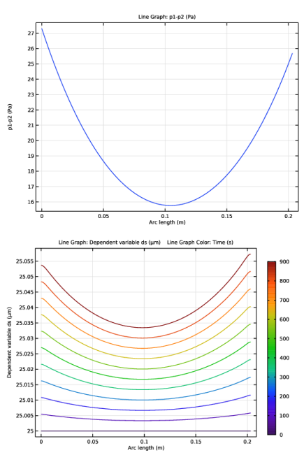
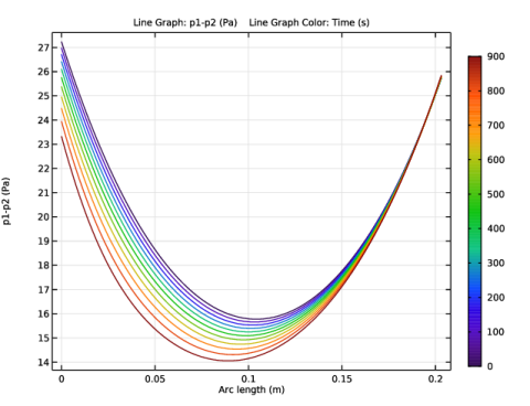
In the Settings window for 1D Plot Group, type Pressure difference along the centerline, without oxidation reaction in the Label text field.
3
Locate the Data section. From the Dataset list, choose Study 1/Parametric Solutions 1 (sol3).
4
From the Parameter selection (Rs_factor) list, choose From list.
5
In the Parameter values (Rs_factor) list, select 0.
6
From the Time selection list, choose From list.
7
In the Times (s) list, select 0.
Line Graph 1
1
Right-click Pressure difference along the centerline, without oxidation reaction and choose Line Graph.
2
3
In the Settings window for Line Graph, locate the y-Axis Data section.
4
In the Expression text field, type p1-p2.
5
In the Pressure difference along the centerline, without oxidation reaction toolbar, click  Plot.
6
Click the  Zoom Extents button in the Graphics toolbar.
Soot layer thickness along the centerline, without oxidation reaction
1
In the Model Builder window, right-click Pressure difference along the centerline, without oxidation reaction and choose Duplicate.
2
In the Settings window for 1D Plot Group, type Soot layer thickness along the centerline, without oxidation reaction in the Label text field.
3
Locate the Data section. From the Time selection list, choose All.
Line Graph 1
1
In the Model Builder window, expand the Soot layer thickness along the centerline, without oxidation reaction node, then click Line Graph 1.
2
In the Settings window for Line Graph, locate the y-Axis Data section.
3
In the Expression text field, type ds.
4
From the Unit list, choose µm.
Color Expression 1
1
Right-click Line Graph 1 and choose Color Expression.
2
In the Settings window for Color Expression, locate the Expression section.
3
In the Expression text field, type t.
4
Click to expand the Title section. From the Title type list, choose Automatic.
5
Click to expand the Coloring and Style section. From the Color table list, choose SpectrumClassic.
6
In the Soot layer thickness along the centerline, without oxidation reaction toolbar, click  Plot.
7
Click the  Zoom Extents button in the Graphics toolbar.
8
Right-click Color Expression 1 and choose Copy.
The following steps create Figure 9 and Figure 10.
Soot layer ds, along the top line
1
In the Home toolbar, click  Add Plot Group and choose 1D Plot Group.
2
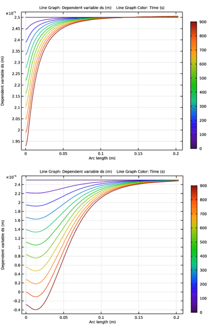
In the Settings window for 1D Plot Group, type Soot layer ds, along the top line in the Label text field.
Line Graph 1
1
Right-click Soot layer ds, along the top line and choose Line Graph.
2
3
In the Settings window for Line Graph, locate the y-Axis Data section.
4
In the Expression text field, type ds.
Color Expression 1
1
Right-click Line Graph 1 and choose Paste Color Expression.
2
In the Soot layer ds, along the top line toolbar, click  Plot.
3
Click the  Zoom Extents button in the Graphics toolbar.
Soot layer ds, along the centerline
1
In the Model Builder window, right-click Soot layer ds, along the top line and choose Duplicate.
2
In the Settings window for 1D Plot Group, type Soot layer ds, along the centerline in the Label text field.
Line Graph 1
1
In the Model Builder window, expand the Soot layer ds, along the centerline node, then click Line Graph 1.
2
In the Settings window for Line Graph, locate the Selection section.
3
Click to select the  Activate Selection toggle button.
4
5
6
In the Soot layer ds, along the centerline toolbar, click  Plot.
Pressure difference p1-p2, along the centerline 1
1
In the Model Builder window, right-click Soot layer ds, along the centerline and choose Duplicate.
2
In the Settings window for 1D Plot Group, type Pressure difference p1-p2, along the centerline 1 in the Label text field.
Line Graph 1
1
In the Model Builder window, expand the Pressure difference p1-p2, along the centerline 1 node, then click Line Graph 1.
2
In the Settings window for Line Graph, locate the y-Axis Data section.
3
In the Expression text field, type p1-p2.
4
In the Pressure difference p1-p2, along the centerline 1 toolbar, click  Plot.