PDF

Precipitation of Barium Sulfate
Introduction
Crystallization is an important separation process in the chemical industry. It is used for the production of pharmaceuticals and industrial chemicals. It can also be used in resource recovery as a way of separating valuable materials from waste. An example of this is the recovery of metals from batteries.
The driving force for crystallization is the amount of solute in excess of its solubility. This is referred to as the supersaturation. Different methods of generating supersaturation are typically used to categorize crystallization processes. These include cooling, evaporation, addition of a secondary solvent (antisolvent), and by chemical reaction (precipitation).
The two main mechanisms that occur during crystallization is nucleation and growth. Nucleation is the formation of new crystal particles in the form of nuclei from solute molecules. Crystal growth is the incorporation of solute molecules into an already existing crystal lattice.
The model is based on the work by Ölander (Ref. 1), Schwarzer and Peukert (Ref. 2), and Tang and others (Ref. 3). The model aims to simulate the evolution of a crystal particle population by solving the population balance equation. The system is modeled both as a perfectly mixed 0D batch reactor and a 3D T-mixer.
Model Definition
The precipitation in 0D is modeled as a time-dependent system where barium chloride and sulphuric acid are assumed perfectly mixed at initial concentrations of 500 and 330 mol/m3. The 3D barium sulfate precipitation takes place in a tubular T-mixer consisting of a 10 mm long mixing pipe with a diameter of 1 mm. Two oppositely placed inlets each with a diameter of 0.5 mm are located at the top of the mixing pipe. The inlets are placed offset from each other. An overview of the geometry can be seen in Figure 1. In 3D, barium chloride and sulphuric acid enter from the oppositely placed inlets at concentrations of 500 and 330 mol/m3. The inlet velocity is adjusted to achieve a Reynolds number of 250 based on the diameter of the mixing pipe. The flow field used for species and particle transport is solved for by the Laminar Flow interface. The T-mixer is modeled at steady state.
Figure 1: T-mixer geometry consisting of two inlet pipes and one main mixing pipe.
In both scenarios, the dissociation of barium chloride and the first step dissociation of sulphuric acid are assumed complete. The second step dissociation of sulphuric acid and formation of aqueous barium sulfate take place according to
while the formation of solid barium sulfate takes place according to
The reactions are set up with the Reaction Engineering interface in 0D and Chemistry interface coupled with the Transport of Diluted Species interface in 3D. The supersaturation is defined as
(1)
where the effective concentration ce and equilibrium concentration c* are calculated from the reactant concentrations using the mean activity coefficient, γ, and the solubility product KSP (mol2/m6) according to
(2)
(3)
Multiple models are available to describe the activity coefficient. Here, the extended Debye–Hückel model presented by Bromley (Ref. 4) is used. The activity coefficient is calculated as
(4)
and
(5)
(6)
where a and c are the anions and cations in the solution. The constants Ba,c are calculated from tabulated values from Bromley (Ref. 4) according to
(7)
For interactions with hydrogen sulfate ions the values are instead taken from and calculations done according to Ref. 3.
The population balance equation
The change in particle number density, n (1/m4), with respect to time in a crystal particle population can be described using the population balance equation
(8)
where
L is the particle diameter (m)
G is the crystal growth rate (m/s)
ν is the kinematic viscosity (m2/s)
Sc is the Schmidt number
B0 the nucleation rate as a source of number density (1/m4/s)
Lc0 the smallest stable crystal size (m)
The terms on the left-hand side represent the change of population density with respect to time, the convective crystal transport, and crystal growth, respectively. The terms on the right-hand side represent the diffusive crystal transport according to Fick’s second law and the birth rate from crystal nucleation. The size distribution is modeled with the population balance equation using the Size‑Based Population Balance interface which solves a discretized formulation with discrete size intervals. The number density ni of a discrete size interval spanning the range Li-1/2 to Li+1/2 is defined as
(9)
The nucleation rate as a source of number density, B0, correlates to the nucleation rate as a source of particle number, B (1/m3/s), as B0 = BL0, where ΔL0 is the width of the interval containing newly formed particles. The rate B is defined according to classical nucleation theory as (Ref. 1, Ref. 3)
(10)
where
DAB is the apparent diffusion coefficient (m2/s)
NA is the Avogadro number (1/mol)
γS is the interfacial energy (J/m2)
kB is the Boltzmann constant (J/K)
Vm is the molecular volume (m3)
T is the temperature (K)
Nucleation occurs at the smallest stable crystal size Lc0 defined as
(11)
with the dissociation number νd. In this model the smallest crystal size at which nucleation occurs is taken as constant. The transport controlled growth rate can be described as (Ref. 3)
(12)
Here ka and kv are the area and volume shape factors relating the particle area and volume to the size, while Sh is the Sherwood number, Mp is the crystal molar mass (kg/mol) and ρp the density of the precipitate (kg/m3).
Reaction rate
The reaction rate, RBaSO4, resulting from the formation of solid barium sulfate, in units of mol/m3/s, is calculated from the summed growth and nucleation source terms of each discrete size interval j according to
(13)
and
(14)
where Vav,j is the average volume of particles and ΔLj is the width of interval j.
When the formation of aqueous barium sulfate is modeled as an equilibrium reaction, where the equilibrium condition is upheld at each point in space and time, the reaction rate can be added either to the aqueous barium sulfate or the barium and sulfate ions. Here, the reaction rate is applied to the aqueous barium sulfate. The reaction rate is added by using the Precipitation in Fluid Flow coupling feature.
Mesh
The mesh is constructed as a tradeoff between computation time and accuracy. The resolution is the highest between the oppositely placed inlets to resolve the mixing of streams. The mesh along the length of the mixing pipe is focused on resolving gradients in the cross-flow direction. Using meshes finer than what this model implements will give more accurate flow fields and crystal growth but require longer times to find a solution.
Results and Discussion
The crystal size distribution for both the perfectly mixed batch reactor and T-mixer scenarios are presented along with complementing data.
Perfectly Mixed Batch Reactor
The supersaturation simultaneously acts as the driving force for the precipitation and represents the amount of available reactant in the solution. The change in supersaturation with time in a perfectly mixed batch reactor is seen in Figure 2. The initial supersaturation is consumed as barium sulfate precipitates until reaching an equilibrium where the ion concentrations are equal to the solubility.
Figure 2: Supersaturation as a function of time in a perfectly mixed batch reactor.
The size distribution of crystals formed from the supersaturation is shown at various times in Figure 3.
Figure 3: Size distribution at various times in a perfectly mixed batch reactor.
The transition from solute reactants to solid particles can be seen from Figure 4, which shows the mass concentrations of the reacting species and the solid product over time. The total concentration remains constant, verifying the conservation of mass in the system.
Figure 4: Mass concentrations of reacting species and solid product over time.
T-Mixer
The total particle concentration, particle flux, and supersaturation in the T-mixer at steady state is shown in Figure 5. The two separate inlet flows mix at the top of the mixing pipe. Along the length of the mixing pipe the combined flow becomes increasingly uniform. The supersaturated state occurs in areas where barium and sulfate ions interact. This is initially at the top part of the mixing pipe. The supersaturated decreases throughout the mixing pipe, indicating nucleation and crystal growth.
Figure 5: Particle Concentration and supersaturation in the T-mixer.
The density distribution at different points along the main mixing channel is shown in Figure 6. The distribution moves towards larger sizes and the total amount of particles increases with retention time.
Figure 6: Number density distribution at various points along the T-mixer main mixing channel.
References
1. M. Ölander, Numerical Simulations for Battery Recycling, master’s thesis, KTH, Royal Institute of Technology, 2023.
2. H.C. Schwarzer and W. Peukert, “Combined experimental/numerical study on the precipitation of nanoparticles,” AICHE J., vol. 50, no. 12, pp. 3234–3247, 2004.
3. H.Y. Tang, S. Rigopoulos, and G. Papadakis, “On the interaction of turbulence with nucleation and growth in reaction crystallisation,” J. Fluid Mech, vol. 944, p. A48, 2022.
4. L.A. Bromley, “Thermodynamic properties of strong electrolytes in aqueous solution”, AICHE J., vol. 19, no. 2, pp. 313–320, 1973.
Application Library path: Chemical_Reaction_Engineering_Module/Mixing_and_Separation/barium_sulfate_precipitation
Modeling Instructions
From the File menu, choose New.
New
In the New window, click  Model Wizard.
Model Wizard
1
In the Model Wizard window, click  0D.
2
In the Select Physics tree, select Chemical Species Transport > Precipitation and Crystallization > Precipitation and Crystallization in Fluid Flow.
3
Click Add.
4
In the Added physics interfaces tree, select Size-Based Population Balance (pbsb).
5
In the Number of population number densities text field, type 100.
6
Click  Study.
7
In the Select Study tree, select General Studies > Time Dependent.
8
Import the parameters for the model from a separate file.
Global Definitions
Parameters 1
1
In the Model Builder window, under Global Definitions click Parameters 1.
2
In the Settings window for Parameters, locate the Parameters section.
3
Click  Load from File.
4
Import the constants for the Debye-Hückel model.
Debye Huckel Constants
1
In the Home toolbar, click  Parameters and choose Add > Parameters.
2
In the Settings window for Parameters, type Debye Huckel Constants in the Label text field.
3
Locate the Parameters section. Click  Load from File.
4
Browse to the model’s Application Libraries folder and double-click the file barium_sulfate_precipitation_debye_huckel_constants.txt.
Ion Interaction
1
In the Home toolbar, click  Functions and choose Global > Analytic.
Define a function to be used for the Debye-Hückel model.
2
In the Settings window for Analytic, type Ion Interaction in the Label text field.
3
In the Function name text field, type B_dot.
4
Locate the Definition section. In the Expression text field, type ((0.06+0.6*B)*(Z1*Z2))/((1+I*1.5/(Z1*Z2))^2)+B.
5
In the Arguments text field, type B, Z1, Z2, I.
6
Locate the Units section. In the Function text field, type kg/mol.
7
Definitions
Variables 1
1
In the Definitions toolbar, click  Local Variables.
Import the required variable expressions for the effective concentration.
2
In the Settings window for Variables, locate the Variables section.
3
Click  Load from File.
4
Reaction Engineering (re)
1
In the Model Builder window, under Component 1 (comp1) click Reaction Engineering (re).
2
In the Settings window for Reaction Engineering, locate the Energy Balance section.
3
In the T text field, type T.
Reaction 1
1
In the Reaction Engineering toolbar, click  Reaction.
2
In the Settings window for Reaction, locate the Reaction Formula section.
3
In the Formula text field, type HSO4(-) = H(+) + SO4(2-).
4
Click Apply.
5
Locate the Equilibrium Settings section. In the Kj text field, type k1.
Reaction 2
1
In the Reaction Engineering toolbar, click  Reaction.
2
In the Settings window for Reaction, locate the Reaction Formula section.
3
In the Formula text field, type Ba(++) + SO4(2-) = BaSO4.
4
Click Apply.
5
Locate the Equilibrium Settings section. In the Kj text field, type k2.
Species 1
1
In the Reaction Engineering toolbar, click  Species.
2
In the Settings window for Species, locate the Name section.
3
4
In the Reaction Engineering toolbar, click  Species.
1
In the Settings window for Species, locate the Name section.
2
3
Locate the Type section. From the list, choose Solvent.
Initial Values 1
1
In the Model Builder window, click Initial Values 1.
2
In the Settings window for Initial Values, locate the Volumetric Species Initial Values section.
3
Size-Based Population Balance (pbsb)
1
In the Model Builder window, under Component 1 (comp1) click Size-Based Population Balance (pbsb).
2
In the Settings window for Size-Based Population Balance, locate the Particle Properties section.
3
In the ρp text field, type rho_BaSO4.
4
Locate the Size Intervals section. In the L0 text field, type 0.82[nm].
5
In the LI text field, type 300[nm].
6
Locate the Nucleation section. From the Nucleation rate list, choose Homogeneous nucleation.
7
In the γs text field, type gamma_CL.
8
In the ν text field, type 2.
9
In the T text field, type T.
10
Locate the Growth section. From the Growth rate list, choose Transport controlled.
11
In the Sh text field, type Sh.
Multiphysics
Precipitation in Fluid Flow 1 (pffg1)
1
In the Model Builder window, under Component 1 (comp1) > Multiphysics click Precipitation in Fluid Flow 1 (pffg1).
2
In the Settings window for Precipitation in Fluid Flow, locate the Precipitant section.
3
4
From the c list, choose User defined.
5
6
In the c* text field, type c_eq.
7
In the Ds text field, type D_AB.
Study 1
Step 1: Time Dependent
1
In the Model Builder window, under Study 1 click Step 1: Time Dependent.
2
In the Settings window for Time Dependent, locate the Study Settings section.
3
In the Output times text field, type 0 0.001 range(0.002,2.0e-3,0.06).
Solution 1 (sol1)
1
In the Study toolbar, click  Show Default Solver.
When the variables solved for have different orders of magnitude, you can modify the scaling of the variables to help the solver converge. In this case, expect the population number density of each bin to be over 1e20 while the concentration values will be significantly lower.
2
In the Model Builder window, expand the Solution 1 (sol1) node, then click Dependent Variables 1.
3
In the Settings window for Dependent Variables, locate the Scaling section.
4
From the Method list, choose Manual.
5
In the Scale text field, type 1e20.
6
In the Model Builder window, expand the Study 1 > Solver Configurations > Solution 1 (sol1) > Dependent Variables 1 node, then click Concentration (comp1.ODE1).
7
In the Settings window for State, locate the Scaling section.
8
From the Method list, choose Initial-value based.
Repeat steps 7 and 8 for the remaining concentration variables: Concentration (comp1.ODE2), Concentration (comp1.ODE3), Concentration (comp1.ODE4), Concentration (comp1.ODE5), and Concentration (comp1.ODE6).
9
In the Model Builder window, under Study 1 > Solver Configurations > Solution 1 (sol1) click Time-Dependent Solver 1.
10
In the Settings window for Time-Dependent Solver, locate the General section.
11
From the Times to store list, choose Output times by interpolation.
12
Click  Compute.
Results
Average Size Distribution (pbsb)
1
In the Settings window for 1D Plot Group, locate the Data section.
2
From the Time selection list, choose From list.
3
In the Times (s) list, choose 0.001, 0.002, 0.004, 0.008, 0.016, 0.032, and 0.06.
Line Segments 1
1
In the Model Builder window, expand the Average Size Distribution (pbsb) node, then click Line Segments 1.
2
In the Settings window for Line Segments, click to expand the Coloring and Style section.
3
From the Width list, choose 2.
4
Click to expand the Legends section. Select the Show legends checkbox.
5
In the Average Size Distribution (pbsb) toolbar, click  Plot.
Supersaturation
1
In the Home toolbar, click  Add Plot Group and choose 1D Plot Group.
2
In the Settings window for 1D Plot Group, type Supersaturation in the Label text field.
3
Click to expand the Title section. From the Title type list, choose None.
4
Locate the Plot Settings section.
5
Select the y-axis label checkbox. In the associated text field, type Supersaturation (1).
6
Locate the Legend section. Clear the Show legends checkbox.
Global 1
1
In the Supersaturation toolbar, click  Global.
2
In the Settings window for Global, locate the y-Axis Data section.
3
Click  Clear Table.
4
5
Click to expand the Coloring and Style section. From the Width list, choose 2.
6
In the Supersaturation toolbar, click  Plot.
Mass Balance
1
In the Home toolbar, click  Add Plot Group and choose 1D Plot Group.
2
In the Settings window for 1D Plot Group, type Mass Balance in the Label text field.
3
Locate the Title section. From the Title type list, choose None.
4
Locate the Plot Settings section.
5
Select the y-axis label checkbox. In the associated text field, type Mass Concentration (kg/m<SUP>3</SUP>).
6
Locate the Legend section. From the Position list, choose Upper left.
Global 1
1
In the Mass Balance toolbar, click  Global.
2
In the Settings window for Global, locate the y-Axis Data section.
3
Click  Clear Table.
4
5
Locate the Coloring and Style section. From the Width list, choose 2.
6
Click to expand the Legends section. From the Legends list, choose Manual.
7
8
In the Mass Balance toolbar, click  Plot.
Reaction Engineering (re)
Generate Space-Dependent Model 1
1
In the Reaction Engineering toolbar, click  Generate Space-Dependent Model.
2
In the Settings window for Generate Space-Dependent Model, locate the Physics Interfaces section.
3
Find the Fluid flow subsection. From the list, choose Laminar Flow: New.
4
Locate the Space-Dependent Model Generation section. Click Create/Refresh.
Component 2 (comp2)
In the Model Builder window, click Component 2 (comp2).
Add Physics
1
In the Home toolbar, click  Add Physics to open the Add Physics window.
2
Go to the Add Physics window.
3
In the tree, select Chemical Species Transport > Precipitation and Crystallization > Size-Based Population Balance (pbsb).
4
Click the Add to Component 2 button in the window toolbar.
5
In the Home toolbar, click  Add Physics to close the Add Physics window.
Multiphysics
Reacting Flow, Diluted Species 1 (rfd1)
1
In the Model Builder window, expand the Component 2 (comp2) > Multiphysics node.
2
Right-click Component 2 (comp2) > Multiphysics > Reacting Flow, Diluted Species 1 (rfd1) and choose Delete.
Precipitation in Fluid Flow 1a (pff1)
In the Physics toolbar, click  Multiphysics Couplings and choose Domain > Precipitation in Fluid Flow.
Definitions (comp2)
Effective Concentration
1
In the Home toolbar, click  Variables and choose Local Variables.
2
In the Settings window for Variables, type Effective Concentration in the Label text field.
3
Locate the Variables section. Click  Load from File.
4
Geometry 1(3D)
Cylinder 1 (cyl1)
1
In the Geometry toolbar, click  Cylinder.
2
In the Settings window for Cylinder, locate the Size and Shape section.
3
In the Radius text field, type D/2.
4
In the Height text field, type Lc.
Cylinder 2 (cyl2)
1
In the Geometry toolbar, click  Cylinder.
2
In the Settings window for Cylinder, locate the Size and Shape section.
3
In the Radius text field, type D/4.
4
In the Height text field, type D.
5
Locate the Position section. In the x text field, type -D.
6
In the y text field, type D/4.
7
In the z text field, type Lc-D/4.
8
Locate the Axis section. From the Axis type list, choose x-axis.
Cylinder 3 (cyl3)
1
In the Geometry toolbar, click  Cylinder.
2
In the Settings window for Cylinder, locate the Size and Shape section.
3
In the Radius text field, type D/4.
4
In the Height text field, type D.
5
Locate the Position section. In the y text field, type -D/4.
6
In the z text field, type Lc-D/4.
7
Locate the Axis section. From the Axis type list, choose x-axis.
Work Plane 1 (wp1)
1
In the Geometry toolbar, click  Work Plane.
2
In the Settings window for Work Plane, locate the Plane Definition section.
3
In the z-coordinate text field, type 9[mm].
Work Plane 1 (wp1) > Plane Geometry
In the Model Builder window, click Plane Geometry.
Work Plane 1 (wp1) > Circle 1 (c1)
1
In the Work Plane toolbar, click  Circle.
2
In the Settings window for Circle, locate the Size and Shape section.
3
In the Radius text field, type D/2.
Ignore Faces 1 (igf1)
1
In the Model Builder window, right-click Geometry 1(3D) and choose Virtual Operations > Ignore Faces.
2
On the object fin, select Boundaries 13–15, 17, 18, 23–26, and 29–31 only.
3
In the Geometry toolbar, click  Build All.
Disable the analysis of the geometry as the remaining small geometric details can be kept.
4
In the Model Builder window, click Geometry 1(3D).
5
In the Settings window for Geometry, locate the Cleanup section.
6
Clear the Automatic detection of small details checkbox.
Chemistry (chem)
1
In the Model Builder window, under Component 2 (comp2) click Chemistry (chem).
2
In the Settings window for Chemistry, locate the Mixture Properties section.
3
From the Phase list, choose Liquid.
4
Locate the Species Matching section. Find the Bulk species subsection. In the table, enter the following settings:
To ensure that the species transport equations converge, change the Reaction type from Equilibrium to Reversible with a high forward rate constant.
1: HSO4(-) = H(+) + SO4(2-)
1
In the Model Builder window, expand the Chemistry (chem) node, then click 1: HSO4(-) = H(+) + SO4(2-).
2
In the Settings window for Reaction, locate the Reaction Formula section.
3
From the Reaction type list, choose Reversible.
4
Locate the Rate Constants section. Select the Specify equilibrium constant checkbox.
5
In the kf text field, type 1e5.
2: Ba(++) + SO4(2-) = BaSO4
1
In the Model Builder window, under Component 2 (comp2) > Chemistry (chem) click 2: Ba(++) + SO4(2-) = BaSO4.
2
In the Settings window for Reaction, locate the Reaction Formula section.
3
From the Reaction type list, choose Reversible.
4
Locate the Rate Constants section. Select the Specify equilibrium constant checkbox.
5
In the kf text field, type 1e5.
Species: H2O (Solvent)
1
In the Model Builder window, click Species: H2O (Solvent).
2
In the Settings window for Species, locate the Chemical Formula section.
3
In the ρ text field, type rho_sol.
Transport of Diluted Species (tds)
In the Model Builder window, expand the Component 2 (comp2) > Transport of Diluted Species (tds) node.
Equilibrium Reaction 1, Equilibrium Reaction 2
1
In the Model Builder window, under Component 2 (comp2) > Transport of Diluted Species (tds), Ctrl-click to select Equilibrium Reaction 1 and Equilibrium Reaction 2.
2
Fluid 1
1
In the Model Builder window, under Component 2 (comp2) > Transport of Diluted Species (tds) click Fluid 1.
2
In the Settings window for Fluid, locate the Diffusion section.
3
From the Source list, choose Material.
4
Locate the Model Input section. From the T list, choose User defined. In the associated text field, type T.
5
Locate the Diffusion section. In the DcBa2p text field, type D_species.
6
In the DcSO42m text field, type D_species.
7
In the DcHSO41m text field, type D_species.
8
In the DcH1p text field, type D_species.
9
In the DcCl1m text field, type D_species.
10
In the DcBaSO4 text field, type D_species.
Inflow 1
1
In the Physics toolbar, click  Boundaries and choose Inflow.
2
3
In the Settings window for Inflow, locate the Concentration section.
4
In the c0,cBa2p text field, type cBa_2p_0.
5
In the c0,cCl1m text field, type cCl_1m_0.
Inflow 2
1
In the Physics toolbar, click  Boundaries and choose Inflow.
2
3
In the Settings window for Inflow, locate the Concentration section.
4
In the c0,cH1p text field, type cH_1p_0.
5
In the c0,cHSO41m text field, type cHSO4_1m_0.
6
In the c0,cSO42m text field, type cSO4_2m_0.
Outflow 1
1
In the Physics toolbar, click  Boundaries and choose Outflow.
2
Size-Based Population Balance 2 (pbsb2)
1
In the Model Builder window, under Component 2 (comp2) click Size-Based Population Balance 2 (pbsb2).
2
In the Settings window for Size-Based Population Balance, locate the Particle Properties section.
3
In the ρp text field, type rho_BaSO4.
4
Locate the Size Intervals section. From the Discretization list, choose Geometric.
5
In the L0 text field, type 0.82[nm].
6
In the LI text field, type 600[nm].
7
In the q text field, type 8.
8
Locate the Nucleation section. From the Nucleation rate list, choose Homogeneous nucleation.
9
In the γs text field, type gamma_CL.
10
In the ν text field, type 2.
11
Locate the Growth section. From the Growth rate list, choose Transport controlled.
12
In the Sh text field, type Sh.
13
Click to expand the Dependent Variables section. In the Number of population number densities text field, type 30.
Laminar Flow (spf)
1
Click the  Show More Options button in the Model Builder toolbar.
2
In the Show More Options dialog, in the tree, select the checkbox for the node Physics > Advanced Physics Options.
3
4
In the Model Builder window, under Component 2 (comp2) click Laminar Flow (spf).
5
In the Settings window for Laminar Flow, click to expand the Advanced Settings section.
6
Find the Pseudo time stepping subsection. From the Use pseudo time stepping for stationary equation form list, choose On.
Size-Based Population Balance 2 (pbsb2)
Fluid 1
1
In the Model Builder window, under Component 2 (comp2) > Size-Based Population Balance 2 (pbsb2) click Fluid 1.
2
In the Settings window for Fluid, locate the Model Input section.
3
From the T list, choose User defined. In the associated text field, type T.
4
Locate the Particle Diffusion section. In the D text field, type D_particles.
Inflow 1
1
In the Physics toolbar, click  Boundaries and choose Inflow.
2
Outflow 1
1
In the Physics toolbar, click  Boundaries and choose Outflow.
2
Laminar Flow (spf)
1
In the Model Builder window, expand the Component 2 (comp2) > Laminar Flow (spf) node, then click Laminar Flow (spf).
2
In the Settings window for Laminar Flow, locate the Physical Model section.
3
In the Tref text field, type T.
Inlet 1
1
In the Physics toolbar, click  Boundaries and choose Inlet.
2
In the Settings window for Inlet, locate the Boundary Condition section.
3
From the list, choose Fully developed flow.
4
Locate the Fully Developed Flow section. In the Uav text field, type u_in.
5
Outlet 1
1
In the Physics toolbar, click  Boundaries and choose Outlet.
2
Multiphysics
Precipitation in Fluid Flow 1a (pff1)
1
In the Model Builder window, under Component 2 (comp2) > Multiphysics click Precipitation in Fluid Flow 1a (pff1).
2
In the Settings window for Precipitation in Fluid Flow, locate the Precipitant section.
3
4
From the c list, choose User defined.
5
6
From the Ds list, choose User defined.
7
8
In the c* text field, type c_eq.
9
Locate the Precipitate section. In the Mp text field, type M_BaSO4.
Mesh 1
1
In the Model Builder window, under Component 2 (comp2) click Mesh 1.
2
In the Settings window for Mesh, locate the Sequence Type section.
3
From the list, choose User-controlled mesh.
Size
1
In the Model Builder window, under Component 2 (comp2) > Mesh 1 click Size.
2
In the Settings window for Size, locate the Element Size section.
3
From the Predefined list, choose Normal.
Size 1
In the Model Builder window, right-click Size 1 and choose Disable.
Corner Refinement 1
1
In the Model Builder window, click Corner Refinement 1.
2
In the Settings window for Corner Refinement, locate the Refinement section.
3
In the Element size scaling factor text field, type 0.5.
Free Tetrahedral 1
1
In the Model Builder window, click Free Tetrahedral 1.
2
In the Settings window for Free Tetrahedral, locate the Domain Selection section.
3
From the Geometric entity level list, choose Domain.
4
Swept 1
1
In the Model Builder window, expand the Boundary Layers 1 node.
2
Right-click Mesh 1 and choose Swept.
3
In the Settings window for Swept, locate the Domain Selection section.
4
From the Geometric entity level list, choose Domain.
5
Click  Paste Selection.
6
In the Paste Selection dialog, type 2 3 in the Selection text field.
7
Distribution 1
1
Right-click Swept 1 and choose Distribution.
2
In the Settings window for Distribution, locate the Distribution section.
3
From the Distribution type list, choose Predefined.
4
In the Number of elements text field, type 30.
5
In the Element ratio text field, type 8.
Swept 1
1
In the Model Builder window, click Swept 1.
2
Drag and drop below Free Tetrahedral 1.
3
In the Settings window for Swept, click  Build All.
Study 2
In the Model Builder window, right-click Study 2 and choose Delete.
Add Study
1
In the Study toolbar, click  Add Study to open the Add Study window.
2
Go to the Add Study window.
3
Find the Physics interfaces in study subsection. In the table, clear the Solve checkboxes for Reaction Engineering (re) and Size-Based Population Balance (pbsb).
4
Find the Multiphysics couplings in study subsection. In the table, clear the Solve checkbox for Precipitation in Fluid Flow 1 (pffg1).
5
Find the Studies subsection. In the Select Study tree, select Preset Studies for Selected Multiphysics > Stationary Precipitation in Fluid Flow.
6
Click the Add Study button in the window toolbar.
7
In the Study toolbar, click  Add Study to close the Add Study window.
Study 2
Step 1: Stationary
In the Study toolbar, click  Compute.
Results
Number of Particles and Supersaturation
Follow these steps to create Figure 5.
1
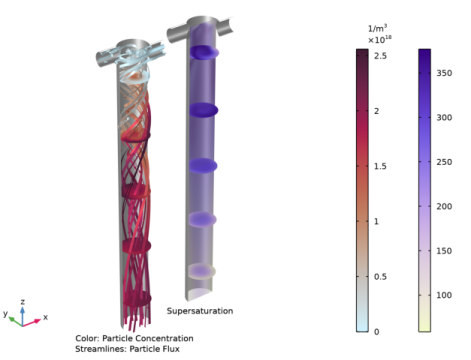
In the Settings window for 3D Plot Group, type Number of Particles and Supersaturation in the Label text field.
2
Click to expand the Title section. From the Title type list, choose None.
3
Locate the Plot Settings section. Clear the Plot dataset edges checkbox.
4
Locate the Color Legend section. Select the Show units checkbox.
5
Click to expand the Plot Array section. Select the Enable checkbox.
Reactor Walls
1
In the Number of Particles and Supersaturation toolbar, click  Surface.
2
In the Settings window for Surface, type Reactor Walls in the Label text field.
3
Locate the Expression section. In the Expression text field, type 1.
4
Click to expand the Plot Array section. Select the Manual indexing checkbox.
Selection 1
1
In the Number of Particles and Supersaturation toolbar, click  Selection.
2
Reactor Walls
In the Model Builder window, click Reactor Walls.
Material Appearance 1
1
In the Number of Particles and Supersaturation toolbar, click  Material Appearance.
2
In the Settings window for Material Appearance, locate the Appearance section.
3
From the Appearance list, choose Custom.
4
From the Material type list, choose Steel (anodized).
Number of Particles and Supersaturation
In the Number of Particles and Supersaturation toolbar, click  Slice.
Slice 1
1
In the Settings window for Slice, locate the Expression section.
2
In the Expression text field, type pbsb2.N.
3
Locate the Plane Data section. From the Plane list, choose xy-planes.
4
Click to expand the Inherit Style section. From the Plot list, choose Streamline 1.
5
Click to expand the Plot Array section. Select the Manual indexing checkbox.
Reactor Walls, Slice 1
1
In the Model Builder window, under Results > Number of Particles and Supersaturation, Ctrl-click to select Reactor Walls and Slice 1.
2
Reactor Walls 1
1
In the Settings window for Surface, locate the Plot Array section.
2
In the Index text field, type 1.
Slice 2
1
In the Model Builder window, click Slice 2.
2
In the Settings window for Slice, locate the Expression section.
3
In the Expression text field, type pbsb2.c/pbsb2.cstar.
4
Locate the Inherit Style section. From the Plot list, choose None.
5
Locate the Coloring and Style section. From the Color table list, choose Baptisia.
6
Locate the Plot Array section. In the Index text field, type 1.
Slice 3
1
Right-click Results > Number of Particles and Supersaturation > Slice 2 and choose Duplicate.
2
In the Settings window for Slice, locate the Plane Data section.
3
From the Plane list, choose zx-planes.
4
In the Planes text field, type 1.
5
Locate the Inherit Style section. From the Plot list, choose Slice 2.
Transparency 1
In the Number of Particles and Supersaturation toolbar, click  Transparency.
Number of Particles and Supersaturation
In the Number of Particles and Supersaturation toolbar, click  Annotation.
Annotation 1
1
In the Settings window for Annotation, locate the Annotation section.
2
In the Text text field, type Color: Particle Concentration \\ Streamlines: Particle Flux.
3
Select the LaTeX markup checkbox.
4
Locate the Position section. In the z text field, type -0.3[mm].
5
Locate the Coloring and Style section. Clear the Show point checkbox.
6
From the Anchor point list, choose Upper middle.
7
Click to expand the Plot Array section. Select the Manual indexing checkbox.
Number of Particles and Supersaturation
In the Number of Particles and Supersaturation toolbar, click  Annotation.
Annotation 2
1
In the Settings window for Annotation, locate the Annotation section.
2
In the Text text field, type Supersaturation.
3
Locate the Position section. In the z text field, type -0.3[mm].
4
Locate the Coloring and Style section. Clear the Show point checkbox.
5
From the Anchor point list, choose Upper middle.
6
Locate the Plot Array section. Select the Manual indexing checkbox.
7
In the Index text field, type 1.
8
In the Number of Particles and Supersaturation toolbar, click  Plot.
Follow these steps to create Figure 6.
Cut Plane 1
1
In the Model Builder window, expand the Results > Datasets node.
2
Right-click Results > Datasets and choose Cut Plane.
3
In the Settings window for Cut Plane, locate the Plane Data section.
4
From the Plane type list, choose General.
5
From the Plane entry method list, choose Point and normal vector.
6
Find the Point subsection. In the z text field, type 5e-3.
Cut Plane 2
1
Right-click Cut Plane 1 and choose Duplicate.
2
In the Settings window for Cut Plane, locate the Plane Data section.
3
Find the Point subsection. In the z text field, type 7.5e-3.
Cut Plane 3
1
Right-click Cut Plane 2 and choose Duplicate.
2
In the Settings window for Cut Plane, locate the Plane Data section.
3
Find the Point subsection. In the z text field, type 8.75e-3.
Cut Plane 4
1
Right-click Cut Plane 3 and choose Duplicate.
2
In the Settings window for Cut Plane, locate the Plane Data section.
3
Find the Point subsection. In the z text field, type 9.375e-3.
Average 3
In the Results toolbar, click  More Datasets and choose Evaluation > Average.
Cut Plane Average 5e-3
1
In the Model Builder window, expand the Results > Population Number Density, n121, Streamline (pbsb2) node, then click Results > Datasets > Average 3.
2
In the Settings window for Average, type Cut Plane Average 5e-3 in the Label text field.
3
Locate the Data section. From the Dataset list, choose Cut Plane 1.
Cut Plane Average 7.5e-3
1
Right-click Cut Plane Average 5e-3 and choose Duplicate.
2
In the Settings window for Average, type Cut Plane Average 7.5e-3 in the Label text field.
3
Locate the Data section. From the Dataset list, choose Cut Plane 2.
Cut Plane Average 8.75e-3
1
Right-click Cut Plane Average 7.5e-3 and choose Duplicate.
2
In the Settings window for Average, type Cut Plane Average 8.75e-3 in the Label text field.
3
Locate the Data section. From the Dataset list, choose Cut Plane 3.
Cut Plane Average 9.375e-3
1
Right-click Cut Plane Average 8.75e-3 and choose Duplicate.
2
In the Settings window for Average, type Cut Plane Average 9.375e-3 in the Label text field.
3
Locate the Data section. From the Dataset list, choose Cut Plane 4.
Average Size Distribution at Specified z-Coordinates
1
In the Model Builder window, under Results click Average Size Distribution at Outlet (pbsb2).
2
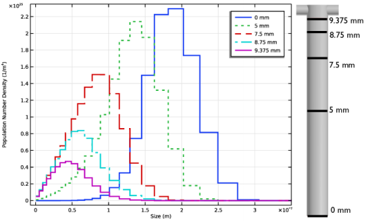
In the Settings window for 1D Plot Group, type Average Size Distribution at Specified z-Coordinates in the Label text field.
3
Locate the Axis section. Select the Manual axis limits checkbox.
4
In the x maximum text field, type 3.5E-7.
Line Segments 1
1
In the Model Builder window, expand the Average Size Distribution at Specified z-Coordinates node, then click Line Segments 1.
2
In the Settings window for Line Segments, click to expand the Coloring and Style section.
3
Find the Line style subsection. From the Line list, choose Cycle.
4
From the Width list, choose 2.
5
Click to expand the Legends section. From the Legends list, choose Manual.
6
Select the Show legends checkbox.
7
Line Segments 2
1
Right-click Results > Average Size Distribution at Specified z-Coordinates > Line Segments 1 and choose Duplicate.
2
In the Settings window for Line Segments, locate the Data section.
3
From the Dataset list, choose Cut Plane Average 5e-3.
4
Locate the Legends section. In the table, enter the following settings:
Line Segments 3
1
Right-click Line Segments 2 and choose Duplicate.
2
In the Settings window for Line Segments, locate the Data section.
3
From the Dataset list, choose Cut Plane Average 7.5e-3.
4
Locate the Legends section. In the table, enter the following settings:
Line Segments 4
1
Right-click Line Segments 3 and choose Duplicate.
2
In the Settings window for Line Segments, locate the Data section.
3
From the Dataset list, choose Cut Plane Average 8.75e-3.
4
Locate the Legends section. In the table, enter the following settings:
Line Segments 5
1
Right-click Line Segments 4 and choose Duplicate.
2
In the Settings window for Line Segments, locate the Data section.
3
From the Dataset list, choose Cut Plane Average 9.375e-3.
4
Locate the Legends section. In the table, enter the following settings:
5
In the Average Size Distribution at Specified z-Coordinates toolbar, click  Plot.
Follow these steps to create the Concentration of Particles at Different Sizes plot found in the model file.
Concentration of Particles at Different Sizes
1
In the Results toolbar, click  3D Plot Group.
2
In the Settings window for 3D Plot Group, type Concentration of Particles at Different Sizes in the Label text field.
3
Locate the Title section. From the Title type list, choose Manual.
4
In the Title text area, type Concentration of Particles at Different Sizes.
5
Locate the Plot Settings section. Clear the Plot dataset edges checkbox.
6
Locate the Color Legend section. Select the Show units checkbox.
7
Locate the Plot Array section. Select the Enable checkbox.
Slice 1
1
In the Concentration of Particles at Different Sizes toolbar, click  Slice.
2
In the Settings window for Slice, locate the Expression section.
3
In the Expression text field, type n105.
4
Locate the Plane Data section. From the Plane list, choose xy-planes.
5
Locate the Plot Array section. Select the Manual indexing checkbox.
Concentration of Particles at Different Sizes
In the Concentration of Particles at Different Sizes toolbar, click  Slice.
Slice 2
1
In the Settings window for Slice, locate the Expression section.
2
In the Expression text field, type n105.
3
Locate the Plane Data section. From the Plane list, choose zx-planes.
4
In the Planes text field, type 1.
5
Locate the Inherit Style section. From the Plot list, choose Slice 1.
6
Locate the Plot Array section. Select the Manual indexing checkbox.
Transparency 1
In the Concentration of Particles at Different Sizes toolbar, click  Transparency.
Concentration of Particles at Different Sizes
In the Concentration of Particles at Different Sizes toolbar, click  Annotation.
Annotation 1
1
In the Settings window for Annotation, locate the Annotation section.
2
In the Text text field, type 20.7 - 26.9 nm.
3
Locate the Position section. In the y text field, type D/2.
4
Locate the Coloring and Style section. Clear the Show point checkbox.
5
Click to expand the Plot Array section. Select the Manual indexing checkbox.
Reactor Walls
In the Model Builder window, under Results > Number of Particles and Supersaturation right-click Reactor Walls and choose Copy.
Reactor Walls
In the Model Builder window, right-click Concentration of Particles at Different Sizes and choose Paste Surface.
Selection 1
1
In the Model Builder window, expand the Reactor Walls node, then click Selection 1.
2
In the Settings window for Selection, locate the Selection section.
3
Click to select the  Activate Selection toggle button.
4
Annotation 1, Reactor Walls, Slice 1, Slice 2
1
In the Model Builder window, under Results > Concentration of Particles at Different Sizes, Ctrl-click to select Slice 1, Slice 2, Annotation 1, and Reactor Walls.
2
Slice 3
1
In the Settings window for Slice, locate the Inherit Style section.
2
From the Plot list, choose Slice 1.
3
Locate the Expression section. In the Expression text field, type n110.
4
Locate the Plot Array section. In the Index text field, type 1.
Slice 4
1
In the Model Builder window, click Slice 4.
2
In the Settings window for Slice, locate the Expression section.
3
In the Expression text field, type n110.
4
Locate the Plot Array section. In the Index text field, type 1.
Annotation 2
1
In the Model Builder window, click Annotation 2.
2
In the Settings window for Annotation, locate the Annotation section.
3
In the Text text field, type 57.6 - 67.1 nm.
4
Locate the Plot Array section. In the Index text field, type 1.
Reactor Walls 1
1
In the Model Builder window, click Reactor Walls 1.
2
In the Settings window for Surface, locate the Plot Array section.
3
In the Index text field, type 1.
Annotation 2, Reactor Walls 1, Slice 3, Slice 4
1
In the Model Builder window, under Results > Concentration of Particles at Different Sizes, Ctrl-click to select Slice 3, Slice 4, Annotation 2, and Reactor Walls 1.
2
Slice 5
1
In the Settings window for Slice, locate the Expression section.
2
In the Expression text field, type n115.
3
Locate the Plot Array section. In the Index text field, type 2.
Slice 6
1
In the Model Builder window, click Slice 6.
2
In the Settings window for Slice, locate the Expression section.
3
In the Expression text field, type n115.
4
Locate the Plot Array section. In the Index text field, type 2.
Annotation 3
1
In the Model Builder window, click Annotation 3.
2
In the Settings window for Annotation, locate the Annotation section.
3
In the Text text field, type 115 - 129 nm.
4
Locate the Plot Array section. In the Index text field, type 2.
Reactor Walls 1.1
1
In the Model Builder window, click Reactor Walls 1.1.
2
In the Settings window for Surface, locate the Plot Array section.
3
In the Index text field, type 2.
Annotation 3, Reactor Walls 1.1, Slice 5, Slice 6
1
In the Model Builder window, under Results > Concentration of Particles at Different Sizes, Ctrl-click to select Slice 5, Slice 6, Annotation 3, and Reactor Walls 1.1.
2
Slice 7
1
In the Settings window for Slice, locate the Expression section.
2
In the Expression text field, type n120.
3
Locate the Plot Array section. In the Index text field, type 3.
Slice 8
1
In the Model Builder window, click Slice 8.
2
In the Settings window for Slice, locate the Expression section.
3
In the Expression text field, type n120.
4
Locate the Plot Array section. In the Index text field, type 3.
Annotation 4
1
In the Model Builder window, click Annotation 4.
2
In the Settings window for Annotation, locate the Annotation section.
3
In the Text text field, type 202 - 225 nm.
4
Locate the Plot Array section. In the Index text field, type 3.
Reactor Walls 1.1.1
1
In the Model Builder window, click Reactor Walls 1.1.1.
2
In the Settings window for Surface, locate the Plot Array section.
3
In the Index text field, type 3.
Delete some superfluous plot groups.
Concentration, BaSO4, Surface (tds), Concentration, Ba_2p, Surface (tds), Concentration, Cl_1m, Surface (tds), Concentration, HSO4_1m, Surface (tds), Concentration, H_1p, Surface (tds), Population Number Density, n101, Streamline (pbsb2), Population Number Density, n101, Surface (pbsb2), Population Number Density, n111, Streamline (pbsb2), Population Number Density, n111, Surface (pbsb2), Population Number Density, n121, Streamline (pbsb2), Population Number Density, n121, Surface (pbsb2)
1
In the Model Builder window, under Results, Ctrl-click to select Concentration, Ba_2p, Surface (tds), Concentration, BaSO4, Surface (tds), Concentration, Cl_1m, Surface (tds), Concentration, H_1p, Surface (tds), Concentration, HSO4_1m, Surface (tds), Population Number Density, n101, Streamline (pbsb2), Population Number Density, n101, Surface (pbsb2), Population Number Density, n111, Streamline (pbsb2), Population Number Density, n111, Surface (pbsb2), Population Number Density, n121, Streamline (pbsb2), and Population Number Density, n121, Surface (pbsb2).
2
Lastly, use Group nodes to organize the result plots.
Average Size Distribution (pbsb), Concentration (re), Mass Balance, Size Intervals (pbsb), Supersaturation
1
In the Model Builder window, under Results, Ctrl-click to select Concentration (re), Average Size Distribution (pbsb), Size Intervals (pbsb), Supersaturation, and Mass Balance.
2
Perfectly Mixed Batch Reactor
In the Settings window for Group, type Perfectly Mixed Batch Reactor in the Label text field.
Average Size Distribution (pbsb2), Average Size Distribution at Specified z-Coordinates, Concentration of Particles at Different Sizes, Concentration, BaSO4, Streamline (tds), Concentration, Ba_2p, Streamline (tds), Concentration, Cl_1m, Streamline (tds), Concentration, HSO4_1m, Streamline (tds), Concentration, H_1p, Streamline (tds), Number of Particles and Supersaturation, Number of Particles, Surface (pbsb2), Pressure (spf), Size Intervals (pbsb2), Velocity (spf)
1
In the Model Builder window, under Results, Ctrl-click to select Concentration, Ba_2p, Streamline (tds), Concentration, BaSO4, Streamline (tds), Concentration, Cl_1m, Streamline (tds), Concentration, H_1p, Streamline (tds), Concentration, HSO4_1m, Streamline (tds), Velocity (spf), Pressure (spf), Number of Particles and Supersaturation, Number of Particles, Surface (pbsb2), Size Intervals (pbsb2), Average Size Distribution (pbsb2), Average Size Distribution at Specified z-Coordinates, and Concentration of Particles at Different Sizes.
2
T-Mixer
In the Settings window for Group, type T-Mixer in the Label text field.