PDF

Large Eddy Simulation of a Sports Car
Introduction
The shape of a car body depends on several factors; besides being appealing, it must also provide comfort and good performance. In the early 20th century, the first two criteria dominated the design. Early versions of the model T resembled motor-driven horse carriages and sometimes even lacked windshield, side-windows, and doors. A later example is the London black cab, which had to be tall enough to comfortably accommodate a passenger wearing a bowler hat and have a turning circle of 25 ft. As the speed of travel increased, performance, both with regard to fuel consumption and stability, became an increasingly important design criterion, leading to the aerodynamically shaped vehicles we see today. The fuel consumption depends on the drag force, which can be obtained, with decent accuracy, from a stationary RANS (Reynolds-averaged Navier–Stokes) simulation. Other important design criteria are related to the fluctuating forces that may induce vibrations causing discomfort to the driver and passengers, and in extreme cases even leading to fatigue of engine and chassis parts. With LES (large eddy simulations), it is possible to resolve the spatially and temporally fluctuating forces acting on a car traveling at high speeds. The fluctuating forces exerted by the flow can be used as surface loads in a structural analysis.
In this model, we perform a LES of a sports car traveling at a speed of 180 km/h. The transient analysis is initialized from the results of a stationary RANS simulation, which in turn has been initialized from a potential-flow solution in order to accelerate the convergence of the RANS simulation.
Model Definition
The car model, which has length L = 4.46 m, width W = 1.92 m, and height H = 1.17 m, is placed inside a block, with length 13L, width 7W and height 10 m, at two car lengths distance from the front face. The model geometry is shown in Figure 1.
Figure 1: Geometry of the computational domain.
The inlet velocity at the front face of the domain, and the velocity of the road (bottom face) is set to U= 50 m/s in the x direction, whereas a slip condition is applied at the side and top faces of the domain. At the rear face of the domain, the gauge pressure is set to zero. On the surfaces of the wheels, the velocity is set to
(1)
where is the unit vector in the direction, is a point on a wheel, is the center of the corresponding wheel, and
(2)
is the magnitude of the angular velocity of the wheels, where Rw is the wheel radius. To model the tire deformation, the road is placed 1 cm up from the lowest point on the tires. The velocity is smoothed exponentially, with a length scale of 2.5 mm, from the tires to the road. Figure 2 shows the magnitude of the applied boundary velocity on the road and front wheel.
Figure 2: Magnitude of velocity in m/s on the road and front wheel boundaries.
The large eddy simulation is initialized from a RANS k-ε solution. In order to accelerate the convergence of the RANS simulation, the k-ε simulation is in turn initialized from a potential-flow solution. For irrotational flow, a velocity potential, ϕ, can be defined such that u = ∇ϕ. Assuming that the flow is incompressible, ϕ can be obtained by solving Laplace’s equation
(3)
with
The initial values for velocity and pressure, applied in the RANS k-ε simulation, are obtained from the potential-flow solution as
The large eddy simulation is first computed for 0.6 s (corresponding to roughly seven car-length passages) to obtain a fully developed turbulent flow field, and after that data is sampled every 2 ms during 0.1 s.
Results and Discussion
Figure 3, Figure 4, and Figure 5 show slice plots of the velocity magnitude for the potential-flow solution, the RANS k-ε solution, and the LES solution at = 0.7 s, respectively. The potential-flow solution quickly approaches its asymptotic state away from the car boundaries; the superposition of a uniform flow and a source doublet. Note that no drag force on the car body can be derived from the potential-flow solution, and thus it is only useful as an initial guess for a more accurate model.
Figure 3: Velocity magnitude in m/s from the potential-flow solution.
The RANS solution has a wake extending all the way to the outlet boundary. This breaking of the fore-aft pressure symmetry (seen in the potential-flow solution) induces a form drag on the car body. The form drag is the major contribution to the total drag on the car.
Figure 4: Velocity magnitude in m/s from the RANS k-ε solution.
Transient vortex detachment can be observed in the LES solution. The drag coefficient, Cd, is given by
(4)
where Fx is the x-component of the force on the car and A is its area cross section:
(5)
where is the shear stress at the wall, ut is the tangential velocity, and the integrations are performed over the surfaces of the car body. The form drag can be obtained by leaving out the shear-stress term in the force calculation.
Figure 5: Velocity magnitude in m/s from the LES solution at t = 0.7 s.
Drag coefficients for the form drag and total drag are shown in Figure 6 as a function of time from = 0.6 s to t = 0.7 s. The (total) drag coefficient fluctuates around the relatively low value of 0.2.
Figure 6: Drag coefficients based on form drag (blue) and total drag (green) from the LES solution between t = 0.6 s and = 0.7 s.
Instantaneous streamlines and slice plots of the velocity magnitude at = 0.7 s are shown in Figure 7 and Figure 8, respectively.
Figure 7: Instantaneous streamlines from the LES solution at = 0.7 s.
Figure 8: Slice plots of the velocity magnitude from the LES solution at = 0.7 s.
The fluctuating surface stresses, obtained from the LES simulation, can be applied as loads in structural analyses of various body parts to look at the excitation of eigenmodes, which can eventually lead to fatigue.
Notes About the COMSOL Implementation
The car body has several simplifications. For example, the cowl panel is neglected, and the different parts of the body are assumed to be assembled perfectly, with no gaps nor misalignments between different body panels. In reality, the body of a real supercar is full of small gaps between body panels and doors, of the order of magnitude of a millimeter. These gaps may induce additional turbulence resulting in a slightly higher drag coefficient. The mesh resolution is purposely made coarse in order to reduce the computation time.
Application Library path: CFD_Module/Single-Phase_Flow/sports_car
Modeling Instructions
From the File menu, choose New.
New
In the New window, click  Model Wizard.
Model Wizard
1
In the Model Wizard window, click  3D.
2
In the Select Physics tree, select Fluid Flow > Single-Phase Flow > Large Eddy Simulation > LES RBVM (spf).
3
Click Add.
4
In the Select Physics tree, select Fluid Flow > Single-Phase Flow > Potential Flow > Incompressible Potential Flow (ipf).
5
Click Add.
6
Click  Study.
7
In the Select Study tree, select Preset Studies for Some Physics Interfaces > Stationary.
8
Define parameters for the moving wall boundary conditions.
Global Definitions
Parameters 1
1
In the Model Builder window, under Global Definitions click Parameters 1.
2
In the Settings window for Parameters, locate the Parameters section.
3
Definitions
Variables 1
1
In the Model Builder window, expand the Component 1 (comp1) > Definitions node.
2
Right-click Definitions and choose Variables.
Define variables for the moving wall conditions (the velocity of the tires).
3
In the Settings window for Variables, locate the Variables section.
4
Set the geometry representation to use the CAD Kernel and activate Design Module Boolean operations.
Geometry 1
1
In the Model Builder window, under Component 1 (comp1) click Geometry 1.
2
In the Settings window for Geometry, locate the Advanced section.
3
From the Geometry representation list, choose CAD kernel.
4
Select the Design Module Boolean operations checkbox.
Insert a geometry sequence that contains the geometry and the selections needed for the boundary selections of the individual surfaces in the geometry.
5
In the Geometry toolbar, click Insert Sequence and choose Insert Sequence.
6
7
In the Geometry toolbar, click  Build All.
8
Click the  Wireframe Rendering button in the Graphics toolbar.
Disable the analysis of the geometry as the remaining small geometric details can be kept.
9
In the Model Builder window, click Geometry 1.
10
Locate the Cleanup section. Clear the Automatic detection of small details checkbox.
11
In the Geometry toolbar, click  Build All.
Materials
In the Model Builder window, under Component 1 (comp1) right-click Materials and choose Browse Materials.
Material Browser
1
In the Material Browser window, select Built-in > Air in the tree.
2
Click  Add to Component.
3
Set the wall treatment to automatic so that wall functions are used where the viscous sublayer is not resolved by the boundary layer mesh.
LES RBVM (spf)
1
In the Model Builder window, under Component 1 (comp1) click LES RBVM (spf).
2
In the Settings window for LES RBVM, locate the Turbulence section.
3
From the Wall treatment list, choose Automatic.
4
Locate the Domain Selection section. Click  Clear Selection.
5
Inlet 1
1
In the Physics toolbar, click  Boundaries and choose Inlet.
2
3
In the Settings window for Inlet, locate the Velocity section.
4
In the U0 text field, type U0.
Outlet 1
1
In the Physics toolbar, click  Boundaries and choose Outlet.
2
Wall 2
1
In the Physics toolbar, click  Boundaries and choose Wall.
2
3
In the Settings window for Wall, locate the Boundary Condition section.
4
From the Wall condition list, choose Slip.
Wall 3
1
In the Physics toolbar, click  Boundaries and choose Wall.
2
3
In the Settings window for Wall, click to expand the Wall Movement section.
4
Select the Sliding wall checkbox.
5
Specify the uw vector as
Wall 4
1
In the Physics toolbar, click  Boundaries and choose Wall.
2
In the Settings window for Wall, locate the Boundary Selection section.
3
From the Selection list, choose Front wheel boundaries.
4
Locate the Wall Movement section. From the Translational velocity list, choose Manual.
5
Specify the utr vector as
Wall 5
1
Right-click Wall 4 and choose Duplicate.
2
In the Settings window for Wall, locate the Boundary Selection section.
3
From the Selection list, choose Rear wheel boundaries.
4
Locate the Wall Movement section. Specify the utr vector as
Set the boundary conditions for the potential flow interface.
Incompressible Potential Flow (ipf)
1
In the Model Builder window, under Component 1 (comp1) click Incompressible Potential Flow (ipf).
2
In the Settings window for Incompressible Potential Flow, locate the Pressure section.
3
In the Uscale text field, type U0.
4
In the Model Builder window, click Incompressible Potential Flow (ipf).
5
Click to expand the Discretization section. From the Velocity potential list, choose Linear.
Velocity 1
1
In the Physics toolbar, click  Boundaries and choose Velocity.
2
3
In the Settings window for Velocity, locate the Velocity section.
4
In the Uin text field, type U0.
Open Boundary 1
1
In the Physics toolbar, click  Boundaries and choose Open Boundary.
2
Mesh 1
1
In the Model Builder window, under Component 1 (comp1) click Mesh 1.
2
In the Settings window for Mesh, locate the Physics-Controlled Mesh section.
3
In the table, clear the Use checkbox for Geometric Analysis, Detail Size.
4
Locate the Sequence Type section. From the list, choose User-controlled mesh.
Size
1
In the Model Builder window, under Component 1 (comp1) > Mesh 1 click Size.
2
In the Settings window for Size, locate the Element Size section.
3
From the Calibrate for list, choose Fluid dynamics.
4
Click the Custom button.
5
Locate the Element Size Parameters section. In the Maximum element size text field, type 0.5.
6
In the Minimum element size text field, type 0.05.
7
In the Maximum element growth rate text field, type 1.11.
Size 1
1
In the Model Builder window, click Size 1.
2
In the Settings window for Size, locate the Element Size section.
3
From the Predefined list, choose Finer.
4
Click the Custom button.
5
Locate the Element Size Parameters section.
6
Select the Maximum element size checkbox. In the associated text field, type 0.3.
7
Select the Minimum element size checkbox. In the associated text field, type 0.05.
Boundary Layer Properties 1
1
In the Model Builder window, expand the Component 1 (comp1) > Mesh 1 > Boundary Layers 1 node, then click Boundary Layer Properties 1.
2
In the Settings window for Boundary Layer Properties, locate the Layers section.
3
In the Number of layers text field, type 5.
4
In the Stretching factor text field, type 1.2.
5
From the Thickness specification list, choose Automatic.
6
In the Thickness adjustment factor text field, type 2.5.
Study 1
Step 1: Stationary
Solve the potential flow equation first by deselecting the LES RBVM (spf) interface in the study settings.
1
In the Model Builder window, under Study 1 click Step 1: Stationary.
2
In the Settings window for Stationary, locate the Physics and Variables Selection section.
3
In the Solve for column of the table, under Component 1 (comp1), clear the checkbox for LES RBVM (spf).
4
In the Study toolbar, click  Compute.
Results
Potential flow
1
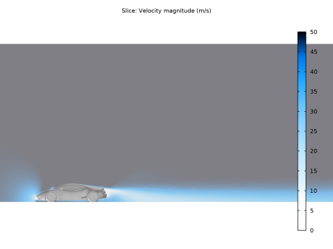
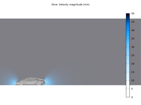
In the Model Builder window, expand the Results node, then click Velocity from Potential Flow Solution (ipf).
2
In the Settings window for 3D Plot Group, type Potential flow in the Label text field.
3
Locate the Plot Settings section. Clear the Plot dataset edges checkbox.
Slice
1
In the Model Builder window, expand the Potential flow node, then click Slice.
2
In the Settings window for Slice, locate the Expression section.
3
In the Expression text field, type ipf.U.
4
Locate the Plane Data section. From the Plane list, choose zx-planes.
5
In the Planes text field, type 1.
Surface 1
1
In the Model Builder window, expand the Results > Potential flow node.
2
Right-click Potential flow and choose Surface.
3
In the Settings window for Surface, locate the Expression section.
4
In the Expression text field, type 1.
5
Locate the Coloring and Style section. From the Coloring list, choose Uniform.
6
From the Color list, choose Gray.
7
Click to expand the Title section. From the Title type list, choose None.
Selection 1
1
Right-click Surface 1 and choose Selection.
2
In the Settings window for Selection, locate the Selection section.
3
From the Selection list, choose Car surfaces.
Slice
1
In the Model Builder window, under Results > Potential flow click Slice.
2
In the Settings window for Slice, locate the Coloring and Style section.
3
From the Color table list, choose JupiterAuroraBorealis.
4
From the Color table transformation list, choose Reverse.
5
Click to expand the Range section. Select the Manual color range checkbox.
6
In the Minimum text field, type 0.
7
In the Maximum text field, type 50.
Transparency 1
1
Right-click Slice and choose Transparency.
2
In the Potential flow toolbar, click  Plot.
To get a better set of initial conditions for the velocity and pressure in the large eddy simulation, add a k-epsilon turbulent interface and solve it on the coarse mesh.
Add Physics
1
In the Home toolbar, click  Add Physics to open the Add Physics window.
2
Go to the Add Physics window.
3
In the tree, select Fluid Flow > Single-Phase Flow > Turbulent Flow > Turbulent Flow, k-ε (spf).
4
Click the Add to Component 1 button in the window toolbar.
5
In the Home toolbar, click  Add Physics to close the Add Physics window.
Turbulent Flow, k-ε 2 (spf2)
1
In the Settings window for Turbulent Flow, k-ε, locate the Domain Selection section.
2
Click  Clear Selection.
3
Copy the boundary conditions in the LES RBVM-interface and paste them into the k-epsilon interface.
LES RBVM (spf)
Inlet 1, Outlet 1, Wall 2, Wall 3, Wall 4, Wall 5
1
In the Model Builder window, under Component 1 (comp1) > LES RBVM (spf), Ctrl-click to select Inlet 1, Outlet 1, Wall 2, Wall 3, Wall 4, and Wall 5.
2
Turbulent Flow, k-ε 2 (spf2)
In the Model Builder window, under Component 1 (comp1) right-click Turbulent Flow, k-ε 2 (spf2) and choose Paste Multiple Items.
Set the initial values for the velocity and the pressure to be computed from the results of the potential flow simulation.
Initial Values 1
1
In the Settings window for Initial Values, locate the Initial Values section.
2
Specify the u vector as
3
In the p text field, type ipf.p.
Add Study
1
In the Home toolbar, click  Add Study to open the Add Study window.
2
Go to the Add Study window.
3
Find the Physics interfaces in study subsection. In the table, clear the Solve checkboxes for LES RBVM (spf) and Incompressible Potential Flow (ipf).
4
Find the Studies subsection. In the Select Study tree, select General Studies > Stationary.
5
Click the Add Study button in the window toolbar.
6
In the Home toolbar, click  Add Study to close the Add Study window.
Study 2
Step 1: Stationary
1
In the Settings window for Stationary, click to expand the Values of Dependent Variables section.
2
Find the Initial values of variables solved for subsection. From the Settings list, choose User controlled.
3
From the Study list, choose Study 1, Stationary.
4
Find the Values of variables not solved for subsection. From the Settings list, choose User controlled.
5
From the Method list, choose Solution.
6
From the Study list, choose Study 1, Stationary.
7
In the Study toolbar, click  Compute.
Results
Slice
1
In the Model Builder window, expand the Results > Velocity (spf2) node, then click Slice.
2
In the Settings window for Slice, locate the Plane Data section.
3
From the Plane list, choose zx-planes.
4
In the Planes text field, type 1.
5
Locate the Coloring and Style section. From the Color table list, choose JupiterAuroraBorealis.
6
From the Color table transformation list, choose Reverse.
7
Click to expand the Range section. Select the Manual color range checkbox.
8
In the Minimum text field, type 0.
9
In the Maximum text field, type 50.
Surface 1
1
In the Model Builder window, expand the Results > Potential flow node.
2
Right-click Surface 1 and choose Copy.
Velocity (spf2)
1
In the Model Builder window, under Results click Velocity (spf2).
2
In the Settings window for 3D Plot Group, locate the Plot Settings section.
3
Clear the Plot dataset edges checkbox.
Surface 1
Right-click Velocity (spf2) and choose Paste Surface.
Transparency 1
1
In the Model Builder window, right-click Slice and choose Transparency.
2
In the Velocity (spf2) toolbar, click  Plot.
Create a finer mesh, to be used in the LES computation, by duplicating Mesh 1 and modifying the settings.
Mesh 1
In the Model Builder window, under Component 1 (comp1) right-click Mesh 1 and choose Duplicate.
Mesh 2
Size
1
In the Model Builder window, expand the Mesh 2 node, then click Size.
2
In the Settings window for Size, locate the Element Size Parameters section.
3
In the Minimum element size text field, type 0.06.
4
In the Maximum element growth rate text field, type 1.13.
5
In the Curvature factor text field, type 0.5.
6
In the Resolution of narrow regions text field, type 0.8.
Size 1
1
In the Model Builder window, click Size 1.
2
In the Settings window for Size, locate the Element Size Parameters section.
3
Select the Maximum element growth rate checkbox.
4
Select the Curvature factor checkbox.
5
Select the Resolution of narrow regions checkbox.
6
In the Minimum element size text field, type 0.1.
7
In the Maximum element growth rate text field, type 1.13.
8
In the Curvature factor text field, type 0.5.
9
In the Resolution of narrow regions text field, type 0.8.
Size 2
1
In the Model Builder window, right-click Mesh 2 and choose Size.
2
Drag and drop Size 2 below Size 1.
3
In the Settings window for Size, locate the Geometric Entity Selection section.
4
From the Geometric entity level list, choose Boundary.
5
From the Selection list, choose Car surfaces.
6
Locate the Element Size section. From the Calibrate for list, choose Fluid dynamics.
7
From the Predefined list, choose Extra fine.
8
Click the Custom button.
9
Locate the Element Size Parameters section.
10
Select the Maximum element size checkbox. In the associated text field, type 0.15.
11
Select the Minimum element size checkbox. In the associated text field, type 0.08.
12
Select the Maximum element growth rate checkbox. In the associated text field, type 1.1.
13
Select the Curvature factor checkbox. In the associated text field, type 0.4.
14
Select the Resolution of narrow regions checkbox. In the associated text field, type 0.9.
Boundary Layer Properties 1
1
In the Model Builder window, expand the Boundary Layers 1 node, then click Boundary Layer Properties 1.
2
In the Settings window for Boundary Layer Properties, locate the Layers section.
3
In the Number of layers text field, type 8.
4
From the Thickness specification list, choose First layer.
5
In the Thickness text field, type 0.003.
Set the initial values in the LES RBVM (spf) interface to correspond to the velocity and pressure calculated with the k-epsilon turbulence model in the previous step.
LES RBVM (spf)
Initial Values 1
1
In the Model Builder window, under Component 1 (comp1) > LES RBVM (spf) click Initial Values 1.
2
In the Settings window for Initial Values, locate the Initial Values section.
3
Specify the u vector as
4
In the p text field, type p2.
Add Study
1
In the Home toolbar, click  Add Study to open the Add Study window.
2
Go to the Add Study window.
3
Find the Studies subsection. In the Select Study tree, select Preset Studies for Some Physics Interfaces > Time Dependent.
4
Find the Physics interfaces in study subsection. In the table, clear the Solve checkboxes for Incompressible Potential Flow (ipf) and Turbulent Flow, k-ε 2 (spf2).
5
Click the Add Study button in the window toolbar.
6
In the Home toolbar, click  Add Study to close the Add Study window.
Study 3
Step 1: Time Dependent
1
In the Settings window for Time Dependent, click to expand the Values of Dependent Variables section.
2
Find the Initial values of variables solved for subsection. From the Settings list, choose User controlled.
3
From the Study list, choose Study 2, Stationary.
4
Find the Values of variables not solved for subsection. From the Settings list, choose User controlled.
5
From the Method list, choose Solution.
6
From the Study list, choose Study 2, Stationary.
7
Locate the Study Settings section. In the Output times text field, type range(0,0.1,0.6), range(0.6,0.002,0.7).
Solution 3 (sol3)
1
In the Study toolbar, click  Show Default Solver.
The variable spf.dt_CFL can be used, but in this case we find that a bit conservative. A constant time step based on the expected maximum velocity and the mesh size in the streamline direction is used instead.
2
In the Model Builder window, expand the Solution 3 (sol3) node.
3
In the Model Builder window, under Study 3 > Solver Configurations > Solution 3 (sol3) click Time-Dependent Solver 1.
4
In the Settings window for Time-Dependent Solver, click to expand the Time Stepping section.
5
From the Steps taken by solver list, choose Free.
6
From the Maximum step constraint list, choose Expression.
7
In the Maximum step text field, type 3e-5.
8
In the Study toolbar, click  Compute.
Results
Velocity (spf)
Change the settings so that the plots are only updated when requested. The plotting takes a while for such large datasets, so when building the plot sequence it is a good idea to turn off the automatic updating of the plots.
1
In the Model Builder window, click Results.
2
In the Settings window for Results, locate the Update of Results section.
3
Select the Only plot when requested checkbox.
Slice
1
In the Model Builder window, expand the Velocity (spf) node, then click Slice.
2
In the Settings window for Slice, locate the Plane Data section.
3
From the Plane list, choose zx-planes.
4
In the Planes text field, type 1.
5
Locate the Coloring and Style section. From the Color table list, choose JupiterAuroraBorealis.
6
From the Color table transformation list, choose Reverse.
7
Click to expand the Range section. Select the Manual color range checkbox.
8
In the Minimum text field, type 0.
9
In the Maximum text field, type 50.
Transparency 1
Right-click Slice and choose Transparency.
Surface 1
1
In the Model Builder window, expand the Results > Velocity (spf2) node.
2
Right-click Surface 1 and choose Copy.
Velocity (spf)
1
In the Model Builder window, under Results click Velocity (spf).
2
In the Settings window for 3D Plot Group, locate the Plot Settings section.
3
Clear the Plot dataset edges checkbox.
Surface 1
Right-click Velocity (spf) and choose Paste Surface.
Create another plot group and make a plot like in Figure 8.
Car with velocity slices
1
In the Results toolbar, click  3D Plot Group.
2
In the Settings window for 3D Plot Group, locate the Data section.
3
From the Dataset list, choose Study 3/Solution 3 (sol3).
4
In the Label text field, type Car with velocity slices.
Slice 1
1
Right-click Car with velocity slices and choose Slice.
2
In the Settings window for Slice, locate the Plane Data section.
3
From the Plane list, choose zx-planes.
4
In the Planes text field, type 1.
5
Locate the Coloring and Style section. From the Color table list, choose JupiterAuroraBorealis.
Slice 2
1
Right-click Slice 1 and choose Duplicate.
2
In the Settings window for Slice, locate the Plane Data section.
3
From the Plane list, choose xy-planes.
4
From the Entry method list, choose Coordinates.
5
In the z-coordinates text field, type .05.
6
Click to expand the Inherit Style section. From the Plot list, choose Slice 1.
7
In the Car with velocity slices toolbar, click  Plot.
Transparency 1
1
In the Model Builder window, expand the Car with velocity slices node.
2
Right-click Slice 1 and choose Transparency.
Slice 2
1
In the Settings window for Slice, click to expand the Title section.
2
From the Title type list, choose None.
Tires
1
In the Model Builder window, right-click Car with velocity slices and choose Surface.
2
In the Settings window for Surface, type Tires in the Label text field.
3
Locate the Expression section. In the Expression text field, type 1.
4
Click to expand the Title section. From the Title type list, choose None.
Selection 1
1
Right-click Tires and choose Selection.
2
In the Settings window for Selection, locate the Selection section.
3
From the Selection list, choose Tires.
Material Appearance 1
1
In the Model Builder window, right-click Tires and choose Material Appearance.
2
In the Settings window for Material Appearance, locate the Appearance section.
3
From the Appearance list, choose Custom.
4
From the Material type list, choose Rubber.
5
From the Color list, choose Black.
Car with velocity slices
1
In the Model Builder window, under Results click Car with velocity slices.
2
In the Settings window for 3D Plot Group, locate the Plot Settings section.
3
Clear the Plot dataset edges checkbox.
Wheel Bays
1
Right-click Car with velocity slices and choose Surface.
2
In the Settings window for Surface, type Wheel Bays in the Label text field.
3
Click to expand the Title section. From the Title type list, choose None.
Selection 1
1
Right-click Wheel Bays and choose Selection.
2
In the Settings window for Selection, locate the Selection section.
3
From the Selection list, choose Wheel bays.
Wheel Bays
1
In the Model Builder window, click Wheel Bays.
2
In the Settings window for Surface, locate the Coloring and Style section.
3
From the Coloring list, choose Uniform.
4
From the Color list, choose Custom.
5
6
Click Define custom colors.
7
8
Click Add to custom colors.
9
Click Show color palette only or OK on the cross-platform desktop.
Windows
1
In the Model Builder window, right-click Tires and choose Duplicate.
2
In the Model Builder window, click Tires 1.
3
In the Settings window for Surface, type Windows in the Label text field.
4
Click to expand the Title section. From the Title type list, choose None.
Selection 1
1
In the Model Builder window, click Selection 1.
2
In the Settings window for Selection, locate the Selection section.
3
From the Selection list, choose Windows.
Material Appearance 1
1
In the Model Builder window, click Material Appearance 1.
2
In the Settings window for Material Appearance, locate the Appearance section.
3
From the Material type list, choose Water.
Headlights
1
In the Model Builder window, right-click Windows and choose Duplicate.
2
In the Settings window for Surface, type Headlights in the Label text field.
3
Click to expand the Title section. From the Title type list, choose None.
Selection 1
1
In the Model Builder window, expand the Headlights node, then click Selection 1.
2
In the Settings window for Selection, locate the Selection section.
3
From the Selection list, choose Headlights.
Material Appearance 1
1
In the Model Builder window, click Material Appearance 1.
2
In the Settings window for Material Appearance, locate the Appearance section.
3
From the Material type list, choose Plastic (shiny).
4
From the Color list, choose White.
Rims
1
In the Model Builder window, right-click Headlights and choose Duplicate.
2
In the Settings window for Surface, type Rims in the Label text field.
3
Click to expand the Title section. From the Title type list, choose None.
Selection 1
1
In the Model Builder window, expand the Rims node, then click Selection 1.
2
In the Settings window for Selection, locate the Selection section.
3
From the Selection list, choose Rims.
Material Appearance 1
1
In the Model Builder window, click Material Appearance 1.
2
In the Settings window for Material Appearance, locate the Appearance section.
3
From the Material type list, choose Rose gold.
Body
1
In the Model Builder window, right-click Rims and choose Duplicate.
2
In the Settings window for Surface, type Body in the Label text field.
3
Click to expand the Title section. From the Title type list, choose None.
Selection 1
1
In the Model Builder window, expand the Body node, then click Selection 1.
2
In the Settings window for Selection, locate the Selection section.
3
From the Selection list, choose Body.
Material Appearance 1
1
In the Model Builder window, click Material Appearance 1.
2
In the Settings window for Material Appearance, in the Graphics window toolbar, clicknext to  Scene Light, then choose Ambient Occlusion.
3
In the Graphics window toolbar, clicknext to  Scene Light, then choose Outdoor Environment.
Rear Lights
1
In the Model Builder window, right-click Body and choose Duplicate.
2
In the Model Builder window, click Body 1.
3
In the Settings window for Surface, type Rear Lights in the Label text field.
4
Click to expand the Title section. From the Title type list, choose None.
Selection 1
1
In the Model Builder window, click Selection 1.
2
In the Settings window for Selection, locate the Selection section.
3
From the Selection list, choose Rear lights.
Material Appearance 1
1
In the Model Builder window, click Material Appearance 1.
2
In the Settings window for Material Appearance, locate the Appearance section.
3
From the Material type list, choose Plastic (shiny).
4
From the Color list, choose Red.
5
In the Car with velocity slices toolbar, click  Plot.
Air vents
1
In the Model Builder window, right-click Wheel Bays and choose Duplicate.
2
In the Settings window for Surface, type Air vents in the Label text field.
3
Click to expand the Title section. From the Title type list, choose None.
Selection 1
1
In the Model Builder window, expand the Air vents node, then click Selection 1.
2
In the Settings window for Selection, locate the Selection section.
3
From the Selection list, choose Air vents.
Air vents
1
In the Model Builder window, click Air vents.
2
In the Settings window for Surface, locate the Coloring and Style section.
3
Click Define custom colors.
4
5
Click Add to custom colors.
6
Click Show color palette only or OK on the cross-platform desktop.
Wheel Bays 1
In the Model Builder window, right-click Wheel Bays and choose Duplicate.
Selection 1
1
In the Model Builder window, expand the Air vents node, then click Selection 1.
2
In the Settings window for Selection, locate the Selection section.
3
From the Selection list, choose Air vents.
Air vents
1
In the Model Builder window, click Air vents.
2
In the Settings window for Surface, type Air vents in the Label text field.
3
In the Car with velocity slices toolbar, click  Plot.
4
Locate the Coloring and Style section. Click Define custom colors.
5
6
Click Add to custom colors.
7
Click Show color palette only or OK on the cross-platform desktop.
8
In the Car with velocity slices toolbar, click  Plot.
Streamlines
1
In the Model Builder window, right-click Car with velocity slices and choose Duplicate.
2
In the Settings window for 3D Plot Group, type Streamlines in the Label text field.
3
In the Model Builder window, expand the Streamlines node.
Slice 1, Slice 2
1
In the Model Builder window, under Results > Streamlines, Ctrl-click to select Slice 1 and Slice 2.
2
Streamline 1
1
In the Model Builder window, right-click Streamlines and choose Streamline.
2
In the Settings window for Streamline, locate the Streamline Positioning section.
3
From the Positioning list, choose Starting-point controlled.
4
From the Entry method list, choose Coordinates.
5
In the x text field, type -8.
6
In the y text field, type 0.
7
In the z text field, type range(0,2/39,2).
8
Locate the Coloring and Style section. Find the Line style subsection. From the Type list, choose Tube.
9
In the Tube radius expression text field, type .005.
10
Select the Radius scale factor checkbox.
11
Click to expand the Advanced section. Clear the Allow backward time integration checkbox.
Color Expression 1
1
Right-click Streamline 1 and choose Color Expression.
2
In the Settings window for Color Expression, click to expand the Range section.
3
Select the Manual color range checkbox.
4
In the Maximum text field, type 70.
5
Locate the Coloring and Style section. From the Color table list, choose RainbowLight.
Streamline 2
1
In the Model Builder window, under Results > Streamlines right-click Streamline 1 and choose Duplicate.
2
In the Settings window for Streamline, locate the Streamline Positioning section.
3
In the x text field, type 4.31.
4
In the y text field, type range(-0.8,0.041025641025641026,0.8).
5
In the z text field, type 0.88.
6
Click to expand the Inherit Style section. From the Plot list, choose Streamline 1.
Streamline 3
1
Right-click Streamline 2 and choose Duplicate.
2
In the Model Builder window, click Streamline 3.
3
In the Settings window for Streamline, locate the Streamline Positioning section.
4
In the z text field, type 0.1.
Streamline 4
1
Right-click Streamline 3 and choose Duplicate.
2
In the Settings window for Streamline, locate the Streamline Positioning section.
3
In the x text field, type -8.
4
In the y text field, type range(-1.5,0.043478260869565216,1.5).
5
In the Streamlines toolbar, click  Plot.
Surface 10
In the Model Builder window, right-click Streamlines and choose Surface.
Selection 1
1
In the Model Builder window, right-click Surface 10 and choose Selection.
2
Material Appearance 1
1
In the Model Builder window, right-click Surface 10 and choose Material Appearance.
2
In the Settings window for Material Appearance, locate the Appearance section.
3
From the Appearance list, choose Custom.
4
From the Material type list, choose Rubber.
5
From the Color list, choose Black.
6
In the Streamlines toolbar, click  Plot.
Visualize the wheel boundary velocity by duplicating the Car with velocity slice plot group, and edit the plot group sequence.
Wheel Velocity
1
In the Model Builder window, right-click Car with velocity slices and choose Duplicate.
2
In the Settings window for 3D Plot Group, type Wheel Velocity in the Label text field.
Slice 1
1
In the Model Builder window, expand the Wheel Velocity node, then click Slice 1.
2
In the Settings window for Slice, locate the Coloring and Style section.
3
Clear the Color legend checkbox.
Slice 2
In the Model Builder window, right-click Slice 2 and choose Disable.
Surface 10
1
In the Model Builder window, right-click Wheel Velocity and choose Surface.
2
In the Settings window for Surface, locate the Expression section.
3
In the Expression text field, type Uwx.
Selection 1
1
Right-click Surface 10 and choose Selection.
2
3
Click the  Zoom Out button in the Graphics toolbar.
4
Click the  Go to XZ View button in the Graphics toolbar.
Rims, Tires
1
In the Model Builder window, under Results > Wheel Velocity, Ctrl-click to select Tires and Rims.
2
Surface 11
In the Model Builder window, right-click Wheel Velocity and choose Surface.
Selection 1
1
In the Model Builder window, right-click Surface 11 and choose Selection.
2
In the Settings window for Selection, locate the Selection section.
3
From the Selection list, choose Front wheel boundaries.
Surface 11
1
In the Model Builder window, click Surface 11.
2
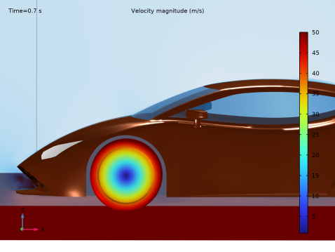
In the Settings window for Surface, click Insert Expression (Ctrl+Space) in the upper-right corner of the Expression section. From the menu, choose Component 1 (comp1) > Definitions > Variables > Uwx - Tire velocity, x-component - m/s.
3
Locate the Expression section. In the Expression text field, type sqrt(Uwx^2+Uwz_front^2).
4
Click to expand the Inherit Style section. From the Plot list, choose Surface 10.
5
In the Wheel Velocity toolbar, click  Plot.
Surface 12
1
In the Model Builder window, right-click Surface 11 and choose Duplicate.
2
In the Settings window for Surface, locate the Expression section.
3
In the Expression text field, type sqrt(Uwx^2+Uwz_rear^2).
4
Click to expand the Inherit Style section. From the Plot list, choose Surface 11.
Selection 1
1
In the Model Builder window, expand the Surface 12 node, then click Selection 1.
2
In the Settings window for Selection, locate the Selection section.
3
From the Selection list, choose Rear wheel boundaries.
Wheel Velocity
1
In the Model Builder window, under Results click Wheel Velocity.
2
In the Settings window for 3D Plot Group, click to expand the Title section.
3
From the Title type list, choose Manual.
4
In the Title text area, type Velocity magnitude (m/s).
5
In the Wheel Velocity toolbar, click  Plot.
To calculate the total drag coefficient, define an integration operator over the surfaces of the car and the wheels, and define variables to calculate the effective exposed area and the drag coefficient, Cd, by following the instructions below. The drag coefficient computed by the pressure only is defined as Cdp. However, we also define a parameter, Cdstress, that includes the viscous stress contributions that can be calculated from the automatic wall functions that are applied wherever the boundary layer is not fully resolved.
Definitions
Integration 1 (intop1)
1
In the Model Builder window, expand the Component 1 (comp1) node.
2
Right-click Component 1 (comp1) > Definitions and choose Nonlocal Couplings > Integration.
3
In the Settings window for Integration, locate the Source Selection section.
4
From the Geometric entity level list, choose Boundary.
5
From the Selection list, choose Car surfaces.
Variables 1
1
In the Model Builder window, click Variables 1.
2
In the Settings window for Variables, locate the Variables section.
3
Study 3
In the Study toolbar, click  Update Solution.
Results
Global Evaluation 1
1
In the Results toolbar, click  Global Evaluation.
2
In the Settings window for Global Evaluation, locate the Data section.
3
From the Dataset list, choose Study 3/Solution 3 (sol3).
4
From the Time selection list, choose From list.
5
In the Times (s) list, choose 0.6 (2), 0.602, 0.604, 0.606, 0.608, 0.61, 0.612, 0.614, 0.616, 0.618, 0.62, 0.622, 0.624, 0.626, 0.628, 0.63, 0.632, 0.634, 0.636, 0.638, 0.64, 0.642, 0.644, 0.646, 0.648, 0.65, 0.652, 0.654, 0.656, 0.658, 0.66, 0.662, 0.664, 0.666, 0.668, 0.67, 0.672, 0.674, 0.676, 0.678, 0.68, 0.682, 0.684, 0.686, 0.688, 0.69, 0.692, 0.694, 0.696, 0.698, and 0.7.
6
Locate the Expressions section. In the table, enter the following settings:
7
Locate the Data Series Operation section. From the Transformation list, choose Average.
8
Click  Evaluate.
Global Evaluation 2
1
In the Model Builder window, right-click Global Evaluation 1 and choose Duplicate.
2
In the Settings window for Global Evaluation, locate the Data Series Operation section.
3
From the Transformation list, choose None.
4
Clicknext to  Evaluate, then choose New Table.
Table 2
1
Go to the Table 2 window.
2
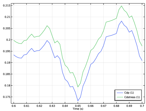
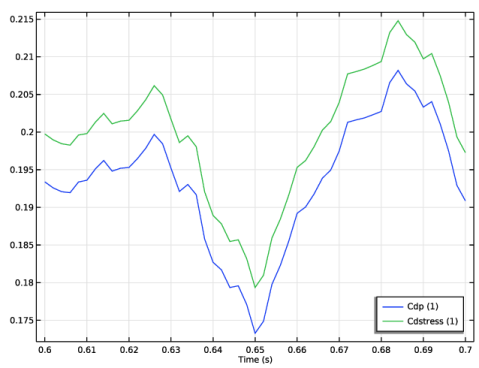
Click the Table Graph button in the window toolbar.
Results
Drag Coefficient
1
In the 1D Plot Group 11 toolbar, click  Plot.
2
In the Settings window for Table Graph, type Drag Coefficient in the Label text field.
3
Click to expand the Legends section. Select the Show legends checkbox.
1D Plot Group 11
1
In the Model Builder window, click 1D Plot Group 11.
2
In the Settings window for 1D Plot Group, locate the Legend section.
3
From the Position list, choose Lower right.
4
In the 1D Plot Group 11 toolbar, click  Plot.