PDF

Jet Pipe
Introduction
This example models the radiation of fan noise from the annular duct of a turbofan aeroengine. When the jet stream excites the duct, a vortex sheet appears along the extension of the duct wall. In the model you calculate the near field on both sides of the vortex sheet. The background mean-flow is assumed to be well described by a potential flow, in this model a uniform flow. This means that, the acoustic field can be modeled by solving the linearized potentiality flow equations in the frequency domain.
Model Definition
The model is axisymmetric with the symmetry axis coinciding with the engine’s centerline (gray area in the figure below). The flows both inside and outside the duct are uniform mean flows, they have a magnitude of M1 and M0, respectively. Because the flow velocities differ, a vortex sheet separates them (dashed line in the figure below).
Sketch of the turbofan motor.
The Linearized Potential Flow, Frequency Domain interface in the Acoustics Module describes acoustic waves in a moving fluid with the potential ϕ, for the local particle velocity as the basic dependent variable; see the chapter about aeroacoustics in the Acoustics Module User’s Guide for details. The field equations are only valid when the background velocity field is irrotational, a condition that is not satisfied across a vortex sheet. As a consequence, the velocity potential is discontinuous across this sheet. To model this discontinuity, you use the Vortex Sheet boundary condition which is available on interior boundaries. The model is excited using the Port boundary condition.
The Vortex Sheet Condition
The Vortex Sheet boundary conditions on the two sides of the vortex sheet are defined as follows:
In these equations, ω is the angular velocity, u0 is the mean-flow velocity, w is the outward normal displacement, ϕ is the velocity potential, and p is the pressure. The subscripts “up” and “down” refer to the two sides of the boundary.
The velocity normal to the vortex sheet is zero, which implies that the last two terms on the left-hand side of the condition vanishes. In the model the variables are made dimensionless. The velocities are divided by the speed of sound in air and the densities are divided by the density for air. For example, the model uses the Mach number M = u0/c0 as the mean flow velocity. This leads to the boundary conditions
where M denotes the transverse Mach number.
The Port Condition
The acoustic field inside the duct can be described as a sum of modes propagating in the duct and then radiating in the free space. This is discussed in section 2.1 in Ref. 1. In this example you study the radiated acoustic waves by exciting the system with a single mode source at a time. The source is introduced using the Port boundary condition with the built-in Annular port option. The port is nonreflecting for the components of the reflected acoustic field that consists of the same modal content. The acoustic field will be reflected due to the impedance change as the outlet of the duct. To get a full nonreflecting behavior several ports need to be added, one for each propagating mode in the system. The mode cutoff frequencies can be evaluated, as done in the first evaluation group in the model. The scattering coefficients associated with the ports are evaluated in the second evaluation group in the model.
Results and Discussion
The inlet sources defined using the Port condition. This example, like Ref. 1, uses the eigenmodes (m,n) = (4,0), (17,1), and (24,1) as incident waves to the duct. In Figure 1 the three source mode pressure fields at the port are depicted in the revolved geometry, including the azimuthal mode contribution.
Figure 1: The incident mode pressures (m,n) = (4,0), (m,n) = (17,1), and (m,n) = (24,1), depicted in the revolved geometry including the azimuthal dependency.
The near-field pressure around the duct obtained by COMSOL Multiphysics can be compared to the results for the near field in Ref. 1. Figure 2 through Figure 6 show the near-field solution for a Mach number equal to M1 = 0.45 in the pipe and M0 = 0.25 on the outside. The figures show the pressure field for the three different source modes.
Figure 2: The near-field solution for m = 4 and n = 0.
Figure 3: The near-field solution for m = 17 and n = 1.
Figure 4: The near-field solution for m = 24 and n = 1.
Figure 5: The near-field sound pressure level for m = 24 and n = 1.
Figure 6: The near-field pressure plotted in the revolved geometry for m = 24 and n = 1.
Reference
1. G. Gabard and R.J. Astley, “Theoretical Model for Sound Radiations from Annular Jet Pipes: Far- and Near-field Solution,” J. Fluid Mech., vol. 549, pp. 315–341, 2006.
Application Library path: Acoustics_Module/Aeroacoustics_and_Noise/jet_pipe
Modeling Instructions
From the File menu, choose New.
New
In the New window, click  Model Wizard.
Model Wizard
1
In the Model Wizard window, click  2D Axisymmetric.
2
In the Select Physics tree, select Acoustics > Aeroacoustics > Linearized Potential Flow, Frequency Domain (lpff).
3
Click Add.
4
Click  Study.
5
In the Select Study tree, select General Studies > Frequency Domain.
6
Root
1
In the Model Builder window, click the root node.
2
In the root node’s Settings window, locate the Unit System section.
3
From the Unit system list, choose None.
This setting turns off all unit support in the model.
Geometry 1
Rectangle 1 (r1)
1
In the Geometry toolbar, click  Rectangle.
2
In the Settings window for Rectangle, locate the Size and Shape section.
3
In the Width text field, type 1.45.
4
In the Height text field, type 1.9.
5
Locate the Position section. In the r text field, type 0.75.
6
In the z text field, type -0.7.
7
Click to expand the Layers section. In the table, enter the following settings:
8
Select the Layers to the right checkbox.
9
Select the Layers on top checkbox.
Rectangle 2 (r2)
1
In the Geometry toolbar, click  Rectangle.
2
In the Settings window for Rectangle, locate the Size and Shape section.
3
In the Width text field, type 0.25.
4
In the Height text field, type 1.9.
5
Locate the Position section. In the r text field, type 0.75.
6
In the z text field, type -0.7.
7
Click to expand the Layers section. In the table, enter the following settings:
Union 1 (uni1)
1
In the Geometry toolbar, click  Booleans and Partitions and choose Union.
2
Click in the Graphics window and then press Ctrl+A to select both objects.
Delete Entities 1 (del1)
1
In the Model Builder window, right-click Geometry 1 and choose Delete Entities.
2
In the Settings window for Delete Entities, locate the Entities or Objects to Delete section.
3
From the Geometric entity level list, choose Domain.
4
On the object uni1, select Domain 1 only.
Form Union (fin)
1
In the Geometry toolbar, click  Build All.
2
Click the  Zoom Extents button in the Graphics toolbar.
This completes the geometry-modeling state. The geometry in the Graphics window should now look like that in the figure below.
3
In the Model Builder window, click Form Union (fin).
Global Definitions
Parameters 1
1
In the Model Builder window, under Global Definitions click Parameters 1.
2
In the Settings window for Parameters, locate the Parameters section.
3
Create three parameter cases to represent the three different source configurations.
4
In the Home toolbar, click  Parameter Case.
5
In the Home toolbar, click  Parameter Case.
6
In the Settings window for Case, locate the Parameters section.
7
8
In the Home toolbar, click  Parameter Case.
9
In the Settings window for Case, locate the Parameters section.
10
Definitions
Port
1
In the Definitions toolbar, click  Explicit.
2
In the Settings window for Explicit, type Port in the Label text field.
3
Locate the Input Entities section. From the Geometric entity level list, choose Boundary.
4
Materials
Specify the density and speed of sound, both normalized to 1, as material parameters.
Material 1 (mat1)
1
In the Model Builder window, under Component 1 (comp1) right-click Materials and choose Blank Material.
2
In the Settings window for Material, locate the Material Contents section.
3
Linearized Potential Flow, Frequency Domain (lpff)
1
In the Model Builder window, under Component 1 (comp1) click Linearized Potential Flow, Frequency Domain (lpff).
2
In the Settings window for Linearized Potential Flow, Frequency Domain, locate the Linearized Potential Flow Equation Settings section.
3
In the m text field, type m.
4
Locate the Global Port Settings section. From the Mode shape normalization list, choose Intensity normalization.
The intensity normalization of the port modes is typically used in aeroacoustic problems with modal source decomposition.
Linearized Potential Flow Model 1
1
In the Model Builder window, under Component 1 (comp1) > Linearized Potential Flow, Frequency Domain (lpff) click Linearized Potential Flow Model 1.
2
In the Settings window for Linearized Potential Flow Model, locate the Model Input section.
3
Specify the u0 vector as
Vortex Sheet 1
1
In the Physics toolbar, click  Boundaries and choose Vortex Sheet.
2
Interior Sound Hard Boundary (Wall) 1
1
In the Physics toolbar, click  Boundaries and choose Interior Sound Hard Boundary (Wall).
2
Linearized Potential Flow Model 2
1
In the Physics toolbar, click  Domains and choose Linearized Potential Flow Model.
2
3
In the Settings window for Linearized Potential Flow Model, locate the Model Input section.
4
Specify the u0 vector as
Port 1
1
In the Physics toolbar, click  Boundaries and choose Port.
2
In the Settings window for Port, locate the Boundary Selection section.
3
From the Selection list, choose Port.
4
Locate the Port Properties section. From the Type of port list, choose Annular.
5
Locate the Port Mode Settings section. In the n text field, type n.
6
Locate the Port Incident Mode Settings section. From the Incident wave excitation at this port list, choose On.
7
From the Define incident wave list, choose Mode scale.
8
In the Sin text field, type 1.
Definitions
Perfectly Matched Layer 1 (pml1)
1
In the Definitions toolbar, click  Perfectly Matched Layer.
2
3
In the Settings window for Perfectly Matched Layer, locate the Geometry section.
4
From the Type list, choose Cylindrical.
5
Locate the Scaling section. From the Coordinate stretching type list, choose Rational.
In this model, the mesh is set up manually. Proceed by directly adding the desired mesh component.
Mesh 1
Free Triangular 1
1
In the Mesh toolbar, click  Free Triangular.
2
In the Settings window for Free Triangular, locate the Domain Selection section.
3
From the Geometric entity level list, choose Domain.
4
Size
1
In the Model Builder window, click Size.
2
In the Settings window for Size, locate the Element Size section.
3
Click the Custom button.
4
Locate the Element Size Parameters section. In the Maximum element size text field, type (1-M1)/f/6.
5
In the Minimum element size text field, type (1-M1)/f/6.
Mapped 1
In the Mesh toolbar, click  Mapped.
Distribution 1
1
Right-click Mapped 1 and choose Distribution.
2
3
In the Settings window for Distribution, locate the Distribution section.
4
In the Number of elements text field, type 8.
5
Click  Build All.
Study 1
1
In the Model Builder window, click Study 1.
2
In the Settings window for Study, locate the Study Settings section.
3
Clear the Generate default plots checkbox.
Step 1: Frequency Domain
1
In the Model Builder window, under Study 1 click Step 1: Frequency Domain.
2
In the Settings window for Frequency Domain, locate the Study Settings section.
3
In the Frequencies text field, type f.
Parametric Sweep
1
In the Study toolbar, click  Parametric Sweep.
2
In the Settings window for Parametric Sweep, locate the Study Settings section.
3
From the Sweep type list, choose Parameter switch.
4
5
In the Study toolbar, click  Compute.
Proceed to plotting the pressure near-field solution shown in Figure 2, Figure 3, and Figure 4.
Results
In the Model Builder window, expand the Results node.
Revolution 2D 1
1
In the Model Builder window, expand the Results > Datasets node.
2
Right-click Results > Datasets and choose Revolution 2D.
3
In the Settings window for Revolution 2D, locate the Data section.
4
From the Dataset list, choose Study 1/Parametric Solutions 1 (sol2).
5
Click to expand the Revolution Layers section. From the Number of layers list, choose Custom.
6
In the Layers text field, type 225.
7
In the Start angle text field, type -90.
8
In the Revolution angle text field, type 225.
9
Click to expand the Advanced section. Select the Define variables checkbox.
Result Templates
1
In the Results toolbar, click  Result Templates to open the Result Templates window.
2
Go to the Result Templates window.
3
In the tree, select Study 1/Parametric Solutions 1 (sol2) > Linearized Potential Flow, Frequency Domain > Acoustic Pressure (lpff).
4
Click the Add Result Template button in the window toolbar.
5
In the Results toolbar, click  Result Templates to close the Result Templates window.
Results
Near-Field Pressure
1
In the Settings window for 2D Plot Group, type Near-Field Pressure in the Label text field.
2
Click to expand the Title section. From the Title type list, choose Manual.
3
In the Title text area, type Near-Field Pressure: (m,n)=(eval(m),eval(n)).
4
Clear the Parameter indicator text field.
5
Click to expand the Selection section. From the Geometric entity level list, choose Domain.
6
7
Locate the Data section. From the Parameters 1 list, choose Case 1.
8
In the Near-Field Pressure toolbar, click  Plot.
9
Click the  Zoom Extents button in the Graphics toolbar.
The graph that appears should be the same as that in Figure 2. Change the parameter cases to generate the graphics in Figure 3 and Figure 4.
10
From the Parameters 1 list, choose Case 2.
11
In the Near-Field Pressure toolbar, click  Plot.
12
From the Parameters 1 list, choose Case 3.
13
In the Near-Field Pressure toolbar, click  Plot.
Create a plot of the sound pressure level as the one shown in Figure 5. Just as for the pressure plot you can change the parameter case to see the other solutions.
Result Templates
1
In the Results toolbar, click  Result Templates to open the Result Templates window.
2
Go to the Result Templates window.
3
In the tree, select Study 1/Parametric Solutions 1 (sol2) > Linearized Potential Flow, Frequency Domain > Sound Pressure Level (lpff).
4
Click the Add Result Template button in the window toolbar.
5
In the Results toolbar, click  Result Templates to close the Result Templates window.
Results
Near-Field SPL
1
In the Settings window for 2D Plot Group, type Near-Field SPL in the Label text field.
2
Click to expand the Title section. From the Title type list, choose Manual.
3
In the Title text area, type Near-Field SPL: (m,n)=(eval(m),eval(n)).
4
Clear the Parameter indicator text field.
5
Click to expand the Selection section. From the Geometric entity level list, choose Domain.
6
Height Expression 1
1
In the Model Builder window, expand the Near-Field SPL node.
2
Right-click Surface and choose Height Expression.
3
In the Near-Field SPL toolbar, click  Plot.
Now, plot the pressure in the revolved geometry including the azimuthal dependency and create Figure 6.
Result Templates
1
In the Results toolbar, click  Result Templates to open the Result Templates window.
2
Go to the Result Templates window.
3
In the tree, select Study 1/Parametric Solutions 1 (sol2) > Linearized Potential Flow, Frequency Domain > Acoustic Pressure, 3D (lpff).
4
Click the Add Result Template button in the window toolbar.
5
In the Results toolbar, click  Result Templates to close the Result Templates window.
Results
Near-Field Pressure, 2D Revolved
1
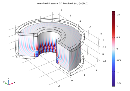
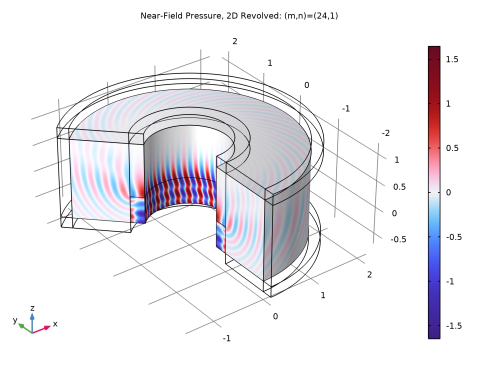
In the Settings window for 3D Plot Group, type Near-Field Pressure, 2D Revolved in the Label text field.
Switch to the previously created Revolution 2D dataset. Note that to capture the azimuthal dependency that dataset is set up to use a fine one degree resolution in the circumferential direction.
2
Locate the Data section. From the Dataset list, choose Revolution 2D 1.
3
Click to expand the Title section. From the Title type list, choose Manual.
4
In the Title text area, type Near-Field Pressure, 2D Revolved: (m,n)=(eval(m),eval(n)).
5
Clear the Parameter indicator text field.
Surface
1
In the Model Builder window, expand the Near-Field Pressure, 2D Revolved node, then click Surface.
2
In the Settings window for Surface, locate the Expression section.
3
In the Expression text field, type lpff.p*exp(-i*m*rev1phi).
Selection 1
1
Right-click Surface and choose Selection.
2
3
In the Near-Field Pressure, 2D Revolved toolbar, click  Plot.
Near-Field Pressure, 2D Revolved 1
In the Model Builder window, right-click Near-Field Pressure, 2D Revolved and choose Duplicate.
Surface
1
In the Model Builder window, expand the Near-Field Pressure, 2D Revolved 1 node, then click Surface.
2
In the Settings window for Surface, locate the Expression section.
3
In the Expression text field, type lpff.p_in_1*exp(-i*m*rev1phi).
Incident Source Mode Pressure
1
In the Model Builder window, under Results click Near-Field Pressure, 2D Revolved 1.
2
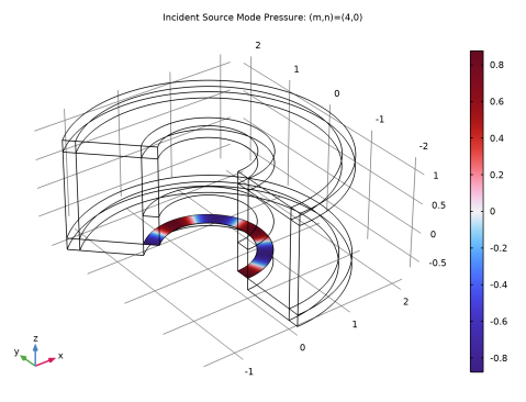
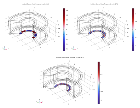
In the Settings window for 3D Plot Group, type Incident Source Mode Pressure in the Label text field.
3
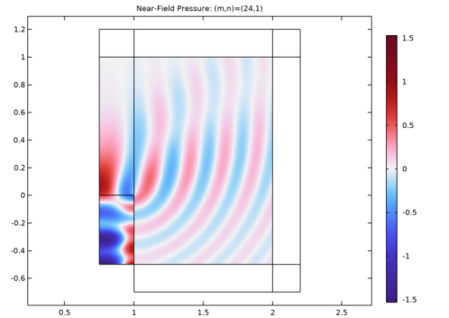
Click to expand the Title section. In the Title text area, type Incident Source Mode Pressure: (m,n)=(eval(m),eval(n)).
4
Locate the Data section. From the Parameters 1 list, choose Case 1.
5
In the Incident Source Mode Pressure toolbar, click  Plot.
6
From the Parameters 1 list, choose Case 2.
7
In the Incident Source Mode Pressure toolbar, click  Plot.
8
From the Parameters 1 list, choose Case 3.
9
In the Incident Source Mode Pressure toolbar, click  Plot.
Finally, evaluate some important quantities like the mode cutoff frequency and the scattering coefficients for the port.
Evaluation Group 1 - Mode Cutoff Frequency
1
In the Results toolbar, click  Evaluation Group.
2
In the Settings window for Evaluation Group, type Evaluation Group 1 - Mode Cutoff Frequency in the Label text field.
3
Locate the Data section. From the Dataset list, choose Study 1/Parametric Solutions 1 (sol2).
Global Evaluation 1
1
Right-click Evaluation Group 1 - Mode Cutoff Frequency and choose Global Evaluation.
2
In the Settings window for Global Evaluation, click Replace Expression in the upper-right corner of the Expressions section. From the menu, choose Component 1 (comp1) > Linearized Potential Flow, Frequency Domain > Ports > Port 1 > lpff.port1.fc - Mode cutoff frequency - 1/s.
3
In the Evaluation Group 1 - Mode Cutoff Frequency toolbar, click  Evaluate.
Evaluation Group 2 - Scattering Coefficient
1
In the Results toolbar, click  Evaluation Group.
2
In the Settings window for Evaluation Group, type Evaluation Group 2 - Scattering Coefficient in the Label text field.
3
Locate the Data section. From the Dataset list, choose Study 1/Parametric Solutions 1 (sol2).
Global Evaluation 1
1
Right-click Evaluation Group 2 - Scattering Coefficient and choose Global Evaluation.
2
In the Settings window for Global Evaluation, click Replace Expression in the upper-right corner of the Expressions section. From the menu, choose Component 1 (comp1) > Linearized Potential Flow, Frequency Domain > Ports > lpff.S11 - S11.
3
Locate the Expressions section. In the table, enter the following settings:
4
In the Evaluation Group 2 - Scattering Coefficient toolbar, click  Evaluate.