|
|
|
|
1
|
|
2
|
In the Select Physics tree, select Acoustics > Pressure Acoustics > Pressure Acoustics, Frequency Domain (acpr).
|
|
3
|
Click Add.
|
|
4
|
Click
|
|
5
|
|
6
|
Click
|
|
1
|
|
2
|
|
3
|
|
4
|
|
1
|
|
2
|
|
3
|
|
4
|
|
5
|
Click
|
|
6
|
|
1
|
|
2
|
|
3
|
|
4
|
|
5
|
|
1
|
|
2
|
|
1
|
|
1
|
|
3
|
|
4
|
|
5
|
In the text field, type 0.03.
|
|
6
|
|
1
|
|
2
|
Go to the Add Material window.
|
|
3
|
|
4
|
Click the Add to Component button in the window toolbar.
|
|
5
|
|
1
|
|
3
|
|
4
|
|
5
|
|
1
|
|
3
|
In the Settings window for Exterior Field Calculation, locate the Exterior Field Calculation section.
|
|
4
|
|
1
|
|
1
|
|
2
|
|
3
|
|
4
|
|
5
|
|
6
|
|
7
|
Click
|
|
1
|
|
2
|
|
1
|
|
2
|
|
3
|
|
4
|
Locate the Physics and Variables Selection section. In the Solve for column of the table, under Component 1 (comp1), clear the checkbox for Deformed Geometry.
|
|
5
|
|
1
|
|
2
|
|
1
|
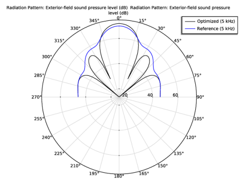
In the Model Builder window, expand the Exterior-Field Sound Pressure Level (acpr) node, then click Radiation Pattern 1.
|
|
2
|
|
3
|
|
1
|
In the Model Builder window, expand the Exterior-Field Pressure (acpr) node, then click Radiation Pattern 1.
|
|
2
|
|
3
|
|
1
|
In the Model Builder window, under Results, Ctrl-click to select Acoustic Pressure (acpr), Sound Pressure Level (acpr), Acoustic Pressure, 3D (acpr), Sound Pressure Level, 3D (acpr), Exterior-Field Sound Pressure Level (acpr), and Exterior-Field Pressure (acpr).
|
|
2
|
Right-click and choose Group.
|
|
1
|
|
2
|
Go to the Add Study window.
|
|
3
|
|
4
|
Click the Add Study button in the window toolbar.
|
|
5
|
|
1
|
|
2
|
|
3
|
|
4
|
|
1
|
|
2
|
|
3
|
|
4
|
Clear the Move limits checkbox.
|
|
5
|
Locate the Objective Function section. In the table, enter the following settings:
|
|
6
|
|
7
|
|
8
|
|
9
|
|
1
|
In the Model Builder window, expand the Study 2 - Optimized Solution > Solver Configurations node, then click Study 2 - Optimized Solution > Step 1: Frequency Domain.
|
|
2
|
|
3
|
|
4
|
|
1
|
|
2
|
In the Model Builder window, expand the Study 2 - Optimized Solution > Solver Configurations > Solution 2 (sol2) > Optimization Solver 1 node, then click Stationary Solver 1.
|
|
3
|
|
4
|
|
5
|
In the Model Builder window, expand the Study 2 - Optimized Solution > Solver Configurations > Solution 2 (sol2) > Optimization Solver 1 > Stationary Solver 1 node, then click Fully Coupled 1.
|
|
6
|
|
7
|
|
1
|
|
2
|
|
3
|
Select the Plot checkbox.
|
|
4
|
|
5
|
|
1
|
|
2
|
|
1
|
|
2
|
|
3
|
|
4
|
|
1
|
In the Model Builder window, expand the Exterior-Field Sound Pressure Level (acpr) 1 node, then click Radiation Pattern 1.
|
|
2
|
|
3
|
|
4
|
|
5
|
|
6
|
|
7
|
|
9
|
|
1
|
Right-click Results > Exterior-Field Sound Pressure Level (acpr) 1 > Radiation Pattern 1 and choose Duplicate.
|
|
2
|
|
3
|
|
4
|
|
5
|
|
6
|
Locate the Legends section. In the table, enter the following settings:
|
|
7
|
|
8
|
|
1
|
In the Model Builder window, expand the Exterior-Field Pressure (acpr) 1 node, then click Radiation Pattern 1.
|
|
2
|
|
3
|
|
1
|
|
2
|
|
3
|
|
1
|
|
2
|
|
3
|
|
1
|
In the Model Builder window, under Results, Ctrl-click to select Acoustic Pressure (acpr) 1, Sound Pressure Level (acpr) 1, Acoustic Pressure, 3D (acpr) 1, Sound Pressure Level, 3D (acpr) 1, Exterior-Field Sound Pressure Level (acpr) 1, Exterior-Field Pressure (acpr) 1, and Shape Optimization.
|
|
2
|
Right-click and choose Group.
|
|
1
|
|
2
|
Go to the Add Study window.
|
|
3
|
|
4
|
Click the Add Study button in the window toolbar.
|
|
5
|
|
1
|
|
2
|
|
3
|
|
4
|
Locate the Physics and Variables Selection section. In the Solve for column of the table, under Component 1 (comp1), clear the checkbox for Deformed Geometry.
|
|
5
|
Click to expand the Values of Dependent Variables section. Find the Values of variables not solved for subsection. From the Settings list, choose User controlled.
|
|
6
|
|
7
|
|
8
|
|
9
|
In the Settings window for Study, type Study 3 - Frequency Sweep (Optimized) in the Label text field.
|
|
10
|
|
11
|
|
1
|
|
2
|
|
3
|
Locate the Data section. From the Dataset list, choose Study 3 - Frequency Sweep (Optimized)/Solution 3 (sol3).
|
|
4
|
Locate the Plot Settings section.
|
|
5
|
|
6
|
|
1
|
|
2
|
|
4
|
|
5
|
|
1
|
|
2
|
|
3
|
|
4
|
Locate the Coloring and Style section. Find the Line style subsection. From the Line list, choose None.
|
|
5
|
|
6
|
|
1
|
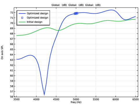
In the Model Builder window, under Results > Optimized solution > Response right-click Global 1 and choose Duplicate.
|
|
2
|
|
3
|
|
4
|
Locate the Legends section. In the table, enter the following settings:
|
|
5
|