|
|
|

|
1
|
|
2
|
In the Select Physics tree, select AC/DC > Electromagnetic Fields > Vector Formulations > Magnetic and Electric Fields (mef).
|
|
3
|
Click Add.
|
|
4
|
In the Select Physics tree, select Mathematics > ODE and DAE Interfaces > Global ODEs and DAEs (ge).
|
|
5
|
Click Add.
|
|
6
|
Click
|
|
7
|
|
8
|
Click
|
|
1
|
|
2
|
|
1
|
|
2
|
|
3
|
|
1
|
|
2
|
|
3
|
|
4
|
|
5
|
|
6
|
Locate the Selections of Resulting Entities section. Select the Resulting objects selection checkbox.
|
|
1
|
|
2
|
|
3
|
|
4
|
|
5
|
Click
|
|
1
|
|
2
|
|
3
|
|
4
|
|
5
|
|
6
|
|
1
|
|
2
|
|
3
|
|
4
|
|
5
|
|
6
|
|
1
|
|
2
|
|
3
|
|
4
|
|
5
|
|
6
|
|
1
|
|
2
|
|
3
|
|
4
|
|
5
|
Select the Keep input objects checkbox.
|
|
6
|
|
7
|
|
8
|
|
1
|
|
2
|
|
4
|
Click
|
|
5
|
|
6
|
|
8
|
|
9
|
|
1
|
|
2
|
|
4
|
|
1
|
In the Model Builder window, right-click Definitions and choose Physics Utilities > Mass Properties.
|
|
2
|
|
3
|
Click
|
|
4
|
|
5
|
|
6
|
|
7
|
|
1
|
|
1
|
|
3
|
In the Settings window for Ampère’s Law and Current Conservation in Solids, locate the Constitutive Relation B-H section.
|
|
4
|
|
5
|
Specify the e vector as
|
|
6
|
|
1
|
|
2
|
In the Settings window for Ampère’s Law and Current Conservation in Solids, locate the Domain Selection section.
|
|
3
|
|
4
|
|
1
|
|
2
|
|
3
|
|
4
|
|
1
|
|
2
|
Go to the Add Material window.
|
|
3
|
|
4
|
Click the Add to Component button in the window toolbar.
|
|
5
|
|
1
|
|
2
|
|
1
|
|
3
|
|
5
|
|
1
|
|
2
|
Go to the Add Material window.
|
|
3
|
In the tree, select AC/DC > Hard Magnetic Materials > Sintered NdFeB Grades (Chinese Standard) > N50 (Sintered NdFeB).
|
|
4
|
Right-click and choose Add to Component 1 (comp1).
|
|
5
|
|
2
|
|
4
|
|
1
|
In the Model Builder window, under Component 1 (comp1) > Global ODEs and DAEs (ge) click Global Equations 1 (ODE1).
|
|
2
|
|
4
|
|
5
|
|
6
|
|
7
|
Click OK.
|
|
8
|
|
9
|
Click
|
|
10
|
|
11
|
|
12
|
Click OK.
|
|
1
|
In the Model Builder window, under Component 1 (comp1) right-click Definitions and choose Variables.
|
|
2
|
|
1
|
|
2
|
In the Settings window for Global Variable Probe, click to expand the Table and Window Settings section.
|
|
3
|
|
1
|
|
2
|
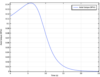
In the Settings window for Global Variable Probe, click Replace Expression in the upper-right corner of the Expression section. From the menu, choose Component 1 (comp1) > Definitions > Variables > axialTorque - Axial torque - N·m.
|
|
3
|
|
1
|
|
2
|
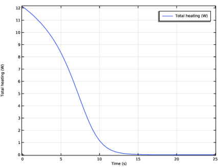
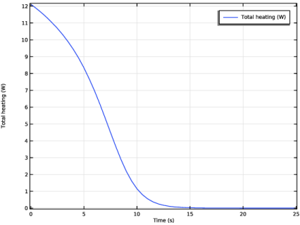
In the Settings window for Global Variable Probe, click Replace Expression in the upper-right corner of the Expression section. From the menu, choose Component 1 (comp1) > Definitions > Variables > totalHeating - Total heating - W.
|
|
3
|
|
1
|
|
2
|
|
1
|
|
2
|
|
3
|
|
4
|
|
1
|
|
2
|
|
3
|
|
4
|
Click
|
|
1
|
|
2
|
|
3
|
In the Solve for column of the table, under Component 1 (comp1), clear the checkbox for Global ODEs and DAEs (ge).
|
|
1
|
|
2
|
|
3
|
|
4
|
|
5
|
|
6
|
Clear the Generate default plots checkbox.
|
|
1
|
|
2
|
|
3
|
|
4
|
|
5
|
|
6
|
|
7
|
|
8
|
Click to expand the Time Stepping section. From the Steps taken by solver list, choose Intermediate.
|
|
9
|
In the Model Builder window, expand the Study 1 > Solver Configurations > Solution 1 (sol1) > Time-Dependent Solver 1 node, then click Iterative 1.
|
|
10
|
|
11
|
|
12
|
|
1
|
|
2
|
|
1
|
|
2
|
|
1
|
|
2
|
|
1
|
|
2
|
|
3
|
Clear the Plot dataset edges checkbox.
|
|
1
|
|
2
|
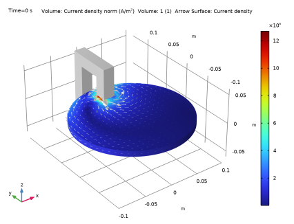
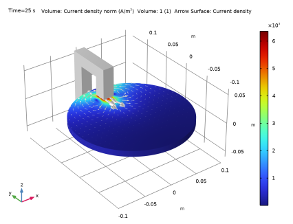
In the Settings window for Volume, click Replace Expression in the upper-right corner of the Expression section. From the menu, choose Component 1 (comp1) > Magnetic and Electric Fields > Currents and charge > mef.normJ - Current density norm - A/m².
|
|
1
|
|
1
|
|
2
|
|
3
|
|
4
|
|
5
|
|
1
|
|
1
|
|
2
|
In the Settings window for Arrow Surface, click Replace Expression in the upper-right corner of the Expression section. From the menu, choose Component 1 (comp1) > Magnetic and Electric Fields > Currents and charge > mef.Jx,mef.Jy,mef.Jz - Current density.
|
|
3
|
|
4
|
|
1
|
|
2
|
|
3
|
|
4
|
|
5
|
|
6
|
|
7
|