|
|
|

|
1
|
|
2
|
Browse to the model’s Application Libraries folder and double-click the file iron_sphere_bfield_00_introduction.mph.
|
|
3
|
|
4
|
Browse to a suitable folder and type the filename iron_sphere_bfield_01_static.mph.
|
|
1
|
|
2
|
|
1
|
|
2
|
|
1
|
|
2
|
|
3
|
|
4
|
|
1
|
In the Model Builder window, expand the Component 1 (comp1) > Mesh 1 > Swept 1 node, then click Distribution 1.
|
|
2
|
|
3
|
|
4
|
Click
|
|
5
|
|
1
|
|
2
|
|
1
|
|
2
|
|
3
|
Select the Auxiliary sweep checkbox.
|
|
4
|
Click
|
|
6
|
|
1
|
|
2
|
|
3
|
|
4
|
|
5
|
|
1
|
|
2
|
|
3
|
|
1
|
|
2
|
|
3
|
|
4
|
|
5
|
|
1
|
|
2
|
|
3
|
|
4
|
|
5
|
|
1
|
|
2
|
|
3
|
|
4
|
|
5
|
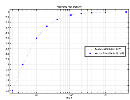
Click to expand the Coloring and Style section. Find the Line style subsection. From the Line list, choose Dotted.
|
|
6
|
|
7
|
|
8
|
|
9
|
|
10
|
|
11
|
Clear the Solution checkbox.
|
|
12
|
Clear the Point checkbox.
|
|
13
|
Select the Unit checkbox.
|
|
14
|
|
1
|
|
2
|
|
3
|
|
4
|
|
5
|
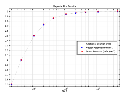
Locate the Coloring and Style section. Find the Line style subsection. From the Line list, choose None.
|
|
6
|
|
7
|
|
8
|
|
9
|
|
10
|
|
11
|
Clear the Solution checkbox.
|
|
12
|
Clear the Point checkbox.
|
|
13
|
Select the Unit checkbox.
|
|
14
|
|
15
|
|
1
|
|
2
|
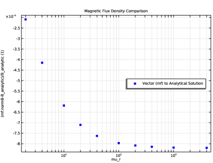
In the Settings window for 1D Plot Group, type Magnetic Flux Density Comparison in the Label text field.
|
|
3
|
|
4
|
|
5
|
|
1
|
|
2
|
|
3
|
|
4
|
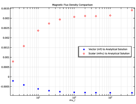
Locate the y-Axis Data section. In the Expression text field, type (mf.normB-B_analytic)/B_analytic.
|
|
5
|
|
6
|
Locate the Coloring and Style section. Find the Line style subsection. From the Line list, choose None.
|
|
7
|
|
8
|
|
9
|
Click to expand the Legends section. In the Label text field, type Vector (mf) to Analytical Solution.
|
|
10
|
|
11
|
|
12
|
Clear the Point checkbox.
|
|
13
|
Clear the Solution checkbox.
|
|
14
|
|
15
|
|
1
|
|
2
|
Go to the Add Physics window.
|
|
3
|
|
4
|
Click the Add to Component 1 button in the window toolbar.
|
|
5
|
|
1
|
In the Settings window for Magnetic Fields, No Currents, locate the Background Magnetic Field section.
|
|
2
|
|
3
|
|
1
|
|
2
|
In the Settings window for Magnetic Flux Conservation in Solids, locate the Domain Selection section.
|
|
3
|
|
1
|
|
1
|
|
2
|
|
3
|
|
4
|
|
5
|
Click
|
|
6
|
|
1
|
|
2
|
|
3
|
In the Solve for column of the table, under Component 1 (comp1), clear the checkbox for Magnetic Fields, No Currents (mfnc).
|
|
1
|
|
2
|
Go to the Add Study window.
|
|
3
|
|
4
|
Click the Add Study button in the window toolbar.
|
|
5
|
|
1
|
|
2
|
|
3
|
Click
|
|
5
|
Locate the Physics and Variables Selection section. In the Solve for column of the table, under Component 1 (comp1), clear the checkbox for Magnetic Fields (mf).
|
|
1
|
|
2
|
|
3
|
|
4
|
|
1
|
|
2
|
|
3
|
|
1
|
|
2
|
|
3
|
|
4
|
|
5
|
|
6
|
|
7
|
Click
|
|
1
|
|
2
|
|
3
|
|
4
|
|
5
|
|
6
|
|
7
|
Locate the Coloring and Style section. Find the Line style subsection. From the Line list, choose None.
|
|
8
|
|
9
|
|
10
|
|
11
|
|
12
|
Clear the Point checkbox.
|
|
13
|
Clear the Solution checkbox.
|
|
14
|
Select the Unit checkbox.
|
|
15
|
|
16
|
|
1
|
|
2
|
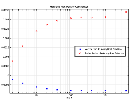
In the Settings window for Point Graph, type Scalar (mfnc) to Analytical Solution in the Label text field.
|
|
3
|
|
4
|
Locate the y-Axis Data section. In the Expression text field, type (mfnc.normB-B_analytic)/B_analytic.
|
|
5
|
Locate the Coloring and Style section. Find the Line style subsection. From the Line list, choose None.
|
|
6
|
|
7
|
|
8
|
|
9
|
|
10
|
Clear the Point checkbox.
|
|
11
|
Clear the Solution checkbox.
|
|
12
|
|
13
|