Contact Angle Boundary Conditions
At a three-phase boundary, it is necessary to add force terms on the boundary to ensure that the fluid maintains a consistent contact angle. Additionally the Wall boundary condition with the Navier Slip option must be used on the walls. The forces acting on the contact point are applied to the model by the Contact Angle node.
Figure 4-4: Forces per unit length acting on a fluid-fluid interface at a three phase boundary with a solid wall. The surface tension force per unit length, σ, is balanced by a reaction force per unit length at the surface, Fn, and by the forces generated by the surface energies of the two phases at the interface: γs1 and γs2.
In equilibrium, the surface tension forces and the normal restoring force from the surface are in balance at a constant contact angle (θc), as shown in Figure 4-4. This equilibrium is expressed by Young’s equation, which considers the components of the forces in the plane of the surface:
(4-26)
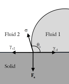
where σ is the surface tension force between the two fluids, γs1 is the surface energy density on the fluid 1 — solid interface and γs2 is the surface energy density on the fluid 2 — solid interface.
There is still debate in the literature as to precisely what occurs in nonequilibrium situations (for example, drop impact) when the physical contact angle deviates from the contact angle specified by a simple application of Young’s equation. A simple approach is to assume that the unbalanced part of the in plane Young Force acts on the fluid to move the contact angle toward its equilibrium value (Ref. 2). COMSOL Multiphysics employs this approach as it is physically motivated and is consistent with the allowed form of the boundary condition from thermodynamics (Ref. 3 and Ref. 4).
The normal force balance at the solid surface is handled by the wall boundary condition, which automatically prevents fluid flow across the solid boundary by the application of a constraint force. The contact angle feature applies a force on the fluid at the interface, fwf, with magnitude:
where θ is the actual contact angle and 
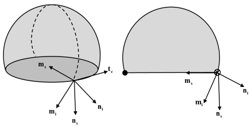
ms is the binormal to the solid surface, as defined in Figure 4-5.
Figure 4-5: Diagram showing normal and tangential vectors defined on the interface between two fluids and a solid surface in 3D (left) and 2D (right). The following vectors are defined: ni, the fluid-fluid interface unit normal; ns, the solid surface unit normal; tc, the tangent to the three-phase contact line; and mi and ms, the two unit binormals, which are defined as mi = tc×ni and ms = tc×ns, respectively.